Diffusion & Flow Matching Part 1: Introduction
- Both diffusion and flow matching learn to transform noise into data
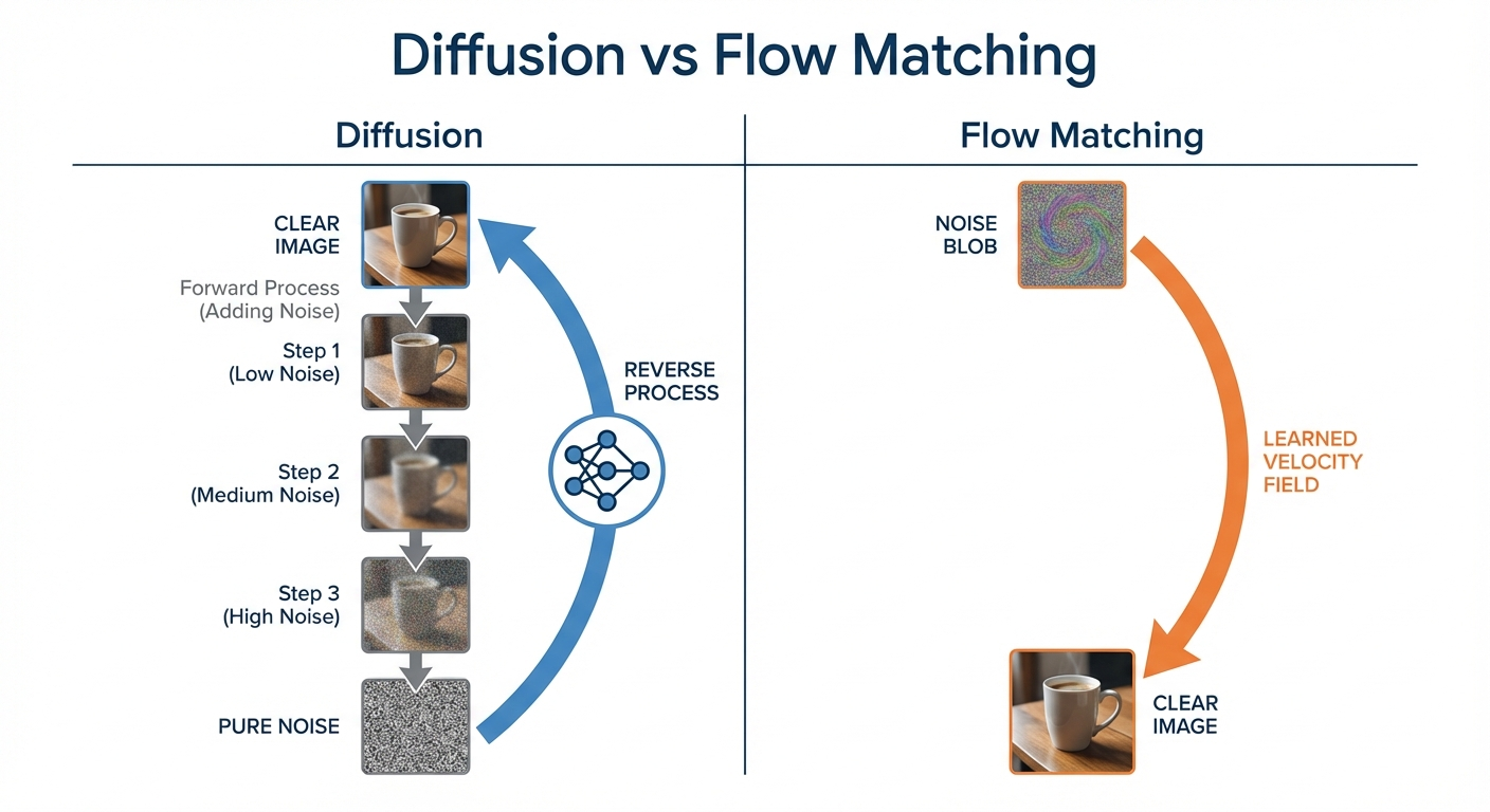
- Flow matching: deterministic ODE trajectories (smooth, predictable paths)
- Diffusion: stochastic SDE trajectories (paths with random perturbations)
- They’re deeply connected — this series develops a unified framework for both
Series Overview
This multi-part series explores the theory behind modern generative models. Each post builds on the previous one:
| Part | Topic | What You’ll Learn |
|---|---|---|
| Part 1 | Introduction (this post) | High-level overview of diffusion and flow matching |
| Part 2 | Understanding Flows | Vector fields, trajectories, and flows — the foundation |
| Part 3 | Probability Paths | How we define paths from noise to data |
| Part 4 | The Flow Matching Loss | The marginalization trick that makes training work |
| Part 5 | Diffusion Models & SDEs | Stochastic differential equations and Brownian motion |
| Part 6 | Score Functions | Conditional and marginal scores, the training trick |
| Part 7 | Training Algorithms | CFM, DDPM, and the conversion formulas |
| Part 8 | Guided Generation | Classifier and classifier-free guidance |
| Part 9 | U-Net Architecture | The workhorse architecture for image generation |
| Part 10 | Diffusion Transformers | DiT: Transformers for diffusion |
| Part 11 | Building an Image Generator | Hands-on: train a flow matching model on CIFAR-10 |
| Part 12 | Why Diffusion? | The multimodal problem — why direct regression fails |
What Are We Building?
Diffusion models and flow matching power today’s best generative AI systems — Stable Diffusion, DALL-E, Midjourney, and Flux. Despite their different formulations, both solve the same fundamental problem:
How do we learn to transform random noise into structured data?
You might wonder: why all this complexity? Can’t we just train a network to map labels to images directly? The short answer is mode averaging — direct regression produces blurry outputs when multiple valid answers exist. See Part 12: Why Diffusion? for the full explanation.
If we can do this, we can generate new images, audio, video, or any data type by starting with random noise and “flowing” toward realistic samples.
Diffusion Models: Adding Stochasticity
Diffusion models work just like flow matching — they learn to transport noise into data — but with one key addition: random perturbations during sampling.
Think of it this way: flow matching follows a smooth, deterministic path from noise to data. Diffusion adds small random “jitters” at each step, like a leaf floating downstream while also being buffeted by turbulence. Both end up at the same destination (the data distribution), but diffusion takes a noisier route.
If you read early diffusion papers (DDPM, 2020), you’ll see a different framing: “add noise to data, then learn to reverse.” This describes the same math with flipped time:
| Convention | t=0 | t=1 | Generation direction |
|---|---|---|---|
| DDPM (2020) | Data | Noise | Reverse: t=1 → t=0 |
| Flow matching (2022+) | Noise | Data | Forward: t=0 → t=1 |
These are mathematically equivalent — just substitute τ = 1−t to convert. This series uses the flow matching convention (t=0 = noise, t=1 = data) because it’s more intuitive: generation “flows forward” from noise to data. Modern systems like Stable Diffusion 3 and FLUX also use this convention.
Flow Matching: The Deterministic Path
Flow matching learns a vector field that tells each point which direction to move:
- Define a path: Specify how to smoothly interpolate between noise and data
- Learn the velocity: Train a neural network to predict the direction of motion along this path
Imagine dropping a leaf into a river. The current tells the leaf which way to move at each moment. If we design the currents correctly, leaves dropped anywhere in the “noise region” will flow toward the “data region.”
The simplest path is a straight line between a noise sample and a data sample. The network learns the velocity field that produces these straight-line trajectories. At generation time, we start from random noise and follow the learned flow — a deterministic ODE that produces the same output every time for a given starting point.
How Do They Compare?
| Aspect | Flow Matching | Diffusion |
|---|---|---|
| Dynamics | ODE (deterministic) | SDE (stochastic) |
| Trajectories | Smooth, predictable paths | Paths with random perturbations |
| What it learns | Velocity field | Velocity field + score function |
| Sampling | Integrate ODE forward | Simulate SDE forward |
| Key advantage | Simpler, often faster | Better sample diversity |
The Deep Connection
Diffusion and flow matching aren’t just related — they’re two views of the same underlying mathematics. Every diffusion model has an equivalent deterministic ODE formulation (the “probability flow ODE”), and every flow matching model can be extended with stochasticity.
The score function ∇ log p_t(x) in diffusion and the velocity field u_t(x) in flow matching are directly related through a conversion formula (derived in Part 7). Train one, and you can compute the other.
This deep connection means you can mix and match: train with the simpler flow matching loss, then sample with the SDE for better diversity. Modern systems like Stable Diffusion 3 do exactly this.
We’ve seen two approaches to generative modeling that are more alike than different. Both flow matching and diffusion learn to transform noise (t=0) into data (t=1). The key difference: flow matching follows deterministic ODE paths, while diffusion adds stochasticity via SDEs.
This series develops a unified framework for both. We’ll build up the theory piece by piece: first understanding what flows are (Part 2), then constructing probability paths (Part 3), deriving training losses (Part 4), adding stochasticity (Part 5), and finally connecting everything through score functions (Parts 6-7).
What’s Next?
In the following posts, we’ll develop the mathematical machinery to understand these methods properly:
- Part 2: We’ll define what “flows” and “vector fields” actually mean
- Part 3: We’ll see how to construct paths from noise to data
- Part 4: We’ll discover the clever trick that makes training tractable
- Part 5: We’ll add stochasticity to get SDEs and understand Brownian motion
- Part 6: We’ll learn about score functions and the training trick
By the end, you’ll understand not just what these models do, but why they work.