Diffusion & Flow Matching Part 5: Diffusion Models and SDEs
- Diffusion models add stochasticity to the ODE: \(dX_t = u_t(X_t)dt + \sigma_t dW_t\)
- Key insight: We derive SDEs by thinking in terms of infinitesimal updates rather than derivatives
- The Brownian motion term \(dW_t\) represents continuous random perturbations
- Setting \(\sigma_t = 0\) recovers the deterministic ODE from flow matching
Diffusion Models: Adding Stochasticity
In Parts 2-4 (flows, probability paths, training), we developed flow matching — a framework where a neural network learns a vector field \(u_t^\theta(x)\) that transports noise to data via an ODE:
\[ dX_t = u_t^\theta(X_t) \, dt \]
This is elegant, but there’s another approach that dominated generative modeling before flow matching emerged: diffusion models. Instead of following a deterministic path, diffusion models add randomness at each step.
Why would we want randomness? It turns out that stochasticity can help exploration during sampling, improve sample diversity, and connects to a rich mathematical theory. Let’s see how.
The Problem with Derivatives
Before we add stochasticity, let’s revisit how we think about ODEs. The standard formulation uses derivatives:
\[ \frac{d}{dt} X_t = u_t(X_t) \]
This says: “the instantaneous rate of change of \(X_t\) equals the vector field \(u_t\) evaluated at \(X_t\).”
Derivatives are elegant for deterministic systems, but they become problematic when we want to add randomness. A random process doesn’t have a well-defined derivative in the classical sense — the path is too “jagged” due to the random perturbations.
To add stochasticity properly, we need a different way to think about dynamics — one that doesn’t rely on taking derivatives.
From Derivatives to Infinitesimal Updates
Instead of asking “what is the derivative?”, we can ask: “what happens over a small time step \(h\)?”
Starting from the ODE, we can write:
\[ \frac{1}{h}(X_{t+h} - X_t) = u_t(X_t) + R_t(h) \]
where \(R_t(h)\) is an error term that goes to zero as \(h \to 0\).
The error term comes from the definition of the derivative itself. The derivative is defined as a limit: \[ \frac{dX_t}{dt} = \lim_{h \to 0} \frac{X_{t+h} - X_t}{h} \]
When \(h\) is small but not zero, the finite difference is only an approximation to the true derivative: \[ \frac{X_{t+h} - X_t}{h} = \frac{dX_t}{dt} + R_t(h) \]
Since the ODE says \(\frac{dX_t}{dt} = u_t(X_t)\), we get the equation above. The key property is that \(R_t(h) \to 0\) as \(h \to 0\), which is exactly what the limit definition guarantees.
What about SDEs? When we add stochasticity, \(X_t\) becomes a random variable, which means the error \(R_t(h)\) is also random. We can no longer simply say “\(R_t(h) \to 0\)” — we need to specify in what sense a random quantity vanishes.
The rigorous statement uses mean square convergence: \[ \mathbb{E}[\|R_t(h)\|^2]^{1/2} \to 0 \quad \text{as } h \to 0 \]
This says the typical size of the error (measured by root-mean-square) goes to zero. Think of it as: “on average, the error becomes negligible.”
Rearranging:
\[ X_{t+h} = X_t + h \cdot u_t(X_t) + h \cdot R_t(h) \]
This says: “where you end up = where you started + (small step) × (direction) + (small error)”. As \(h \to 0\), the error term vanishes and we recover the ODE behavior.
This infinitesimal update formulation is exactly what we need. It describes the dynamics without ever taking a derivative — we just describe how the state changes over small time intervals.
Adding Stochasticity: The SDE
Now we can add randomness naturally. At each small time step, we add a random perturbation:
\[ X_{t+h} = X_t + \underbrace{h \cdot u_t(X_t)}_{\text{deterministic drift}} + \underbrace{\sigma_t (W_{t+h} - W_t)}_{\text{random perturbation}} + \underbrace{h \cdot R_t(h)}_{\text{error term}} \]
Here:
- \(u_t(X_t)\) is the drift — the deterministic direction (same as in flow matching)
- \(\sigma_t\) is the diffusion coefficient — controls how much randomness we add
- \(W_t\) is Brownian motion — a mathematical model of continuous random motion
- \(W_{t+h} - W_t\) is the random increment over the time interval \([t, t+h]\)
As \(h \to 0\), we write this compactly as the stochastic differential equation (SDE):
\[ dX_t = \textcolor{green}{u_t(X_t)} \, dt + \textcolor{orange}{\sigma_t} \, \textcolor{red}{dW_t} \tag{1}\]
where \(\textcolor{green}{\text{drift}}\) is the deterministic direction (same as flow matching), \(\textcolor{orange}{\text{diffusion coefficient}}\) controls noise strength, and \(\textcolor{red}{\text{Brownian increment}}\) adds randomness.
Notice that we never took a derivative of the random process! The SDE notation \(dX_t\) is shorthand for the infinitesimal update, not an actual derivative. This is why SDEs can describe processes with random, non-differentiable paths.
When \(\sigma_t = 0\), the SDE reduces to an ODE, and we recover flow matching.
A diffusion model is defined by: \[ \begin{aligned} dX_t &= u_t^\theta(X_t) \, dt + \sigma_t \, dW_t && \text{(SDE dynamics)} \\ X_0 &\sim p_{\text{init}} && \text{(random initialization)} \end{aligned} \]
The drift \(u_t^\theta\) is parameterized by a neural network, and \(p_{\text{init}}\) is typically a simple distribution like \(\mathcal{N}(0, I)\). Compare this to flow matching, which has the same structure but with \(\sigma_t = 0\) (no stochasticity).
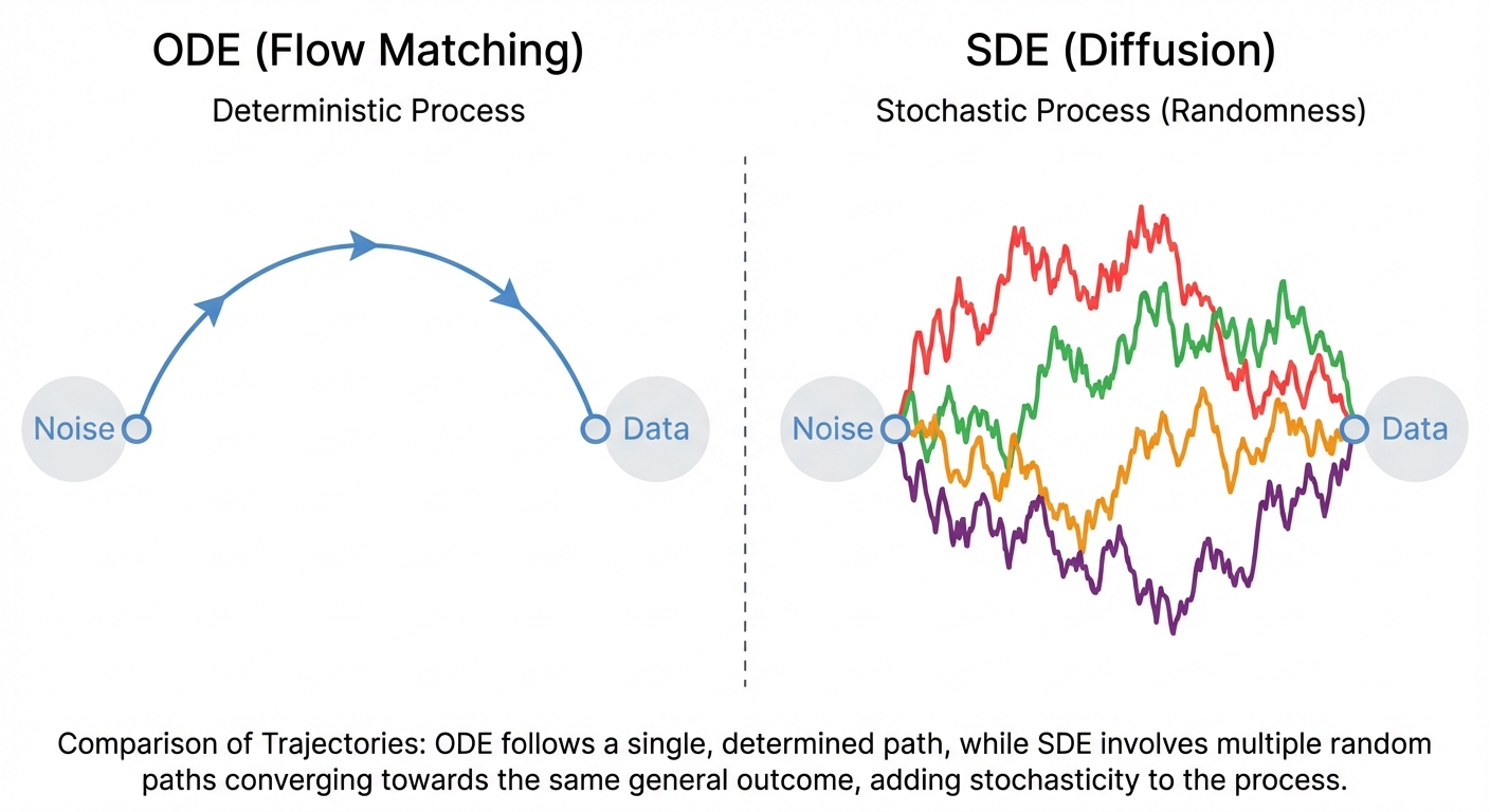
Recall that for ODEs, we had a flow map \(\phi_t\) that deterministically mapped initial points to their positions at time \(t\). SDEs don’t have this! Given a starting point \(X_0\), the value \(X_t\) is no longer fully determined — the stochastic evolution means different runs produce different trajectories. This is a fundamental difference that will affect how we think about probability distributions.
What is Brownian Motion?
Brownian motion \(W_t\) (also called a Wiener process) is the mathematical model of “pure randomness” evolving continuously in time.
Start with something familiar: a random walk. At each step, flip a coin and move +1 or -1. After \(n\) steps, your position is the sum of \(n\) random \(\pm 1\)’s.
Now speed this up: take smaller steps more frequently. If you take \(n\) steps of size \(1/\sqrt{n}\) per unit time, something magical happens as \(n \to \infty\) — you get Brownian motion. The \(\sqrt{n}\) scaling is crucial: it ensures the variance grows linearly with time (not too fast, not too slow).
The result is a continuous path that:
- Never stops jiggling (infinitely many tiny steps)
- Has no preferred direction (mean 0)
- Accumulates uncertainty over time (variance = time elapsed)
Formally, Brownian motion has these properties:
- Starts at zero: \(W_0 = 0\)
- Independent increments: \(W_{t+h} - W_t\) is independent of everything up to time \(t\)
- Gaussian increments: \(W_{t+h} - W_t \sim \mathcal{N}(0, h \cdot I)\)
- Continuous paths: \(W_t\) is continuous in \(t\) (but nowhere differentiable!)
Using these properties, we can simulate an SDE over a small time step. Starting from the SDE: \[ dX_t = u_t(X_t) \, dt + \sigma_t \, dW_t \]
Over a finite step of size \(h\):
- \(dt\) becomes the step size \(h\)
- \(dW_t\) becomes the increment \(W_{t+h} - W_t\)
By the Gaussian increments property, \(W_{t+h} - W_t \sim \mathcal{N}(0, h \cdot I)\). We can sample from this distribution using the reparameterization trick: \[ W_{t+h} - W_t = \sqrt{h} \cdot \epsilon, \quad \epsilon \sim \mathcal{N}(0, I) \]
This works because scaling a \(\mathcal{N}(0, I)\) sample by \(\sqrt{h}\) gives variance \(h\) (since \(\text{Var}(\sqrt{h} \cdot \epsilon) = h \cdot \text{Var}(\epsilon) = h\)).
Putting it together, we get the Euler-Maruyama discretization: \[ X_{t+h} \approx X_t + u_t(X_t) \cdot h + \sigma_t \sqrt{h} \cdot \epsilon, \quad \epsilon \sim \mathcal{N}(0, I) \]
This is the simplest way to simulate an SDE numerically. Notice how the noise scales with \(\sqrt{h}\), not \(h\) — this is a fundamental property of Brownian motion.
The Diffusion Coefficient
The diffusion coefficient \(\sigma_t\) controls the “temperature” of the random noise:
- Large \(\sigma_t\): More exploration, paths spread out quickly
- Small \(\sigma_t\): More deterministic, paths stay close to the drift
- \(\sigma_t = 0\): Pure ODE (flow matching)
In diffusion models, \(\sigma_t\) is typically a schedule that varies with time. Common choices:
| Schedule | \(\sigma_t\) | Used in |
|---|---|---|
| Variance Preserving (VP) | \(\sqrt{\beta_t}\) | DDPM |
| Variance Exploding (VE) | \(\sqrt{\frac{d[\sigma^2(t)]}{dt}}\) | NCSN/NCSNv2 |
| Sub-VP | Interpolation | Score SDE |
The choice of schedule affects sample quality, training stability, and generation speed.
Forward and Reverse Processes
In diffusion models, we typically define:
- Forward process: An SDE that gradually adds noise to data until it becomes pure noise
- Reverse process: An SDE that removes noise, going from noise back to data
The forward process is usually simple and fixed (e.g., just adding Gaussian noise). The challenge is learning to reverse it.
Given the forward SDE that corrupts data into noise, what is the reverse SDE that transforms noise back into data?
It turns out there’s a beautiful mathematical result: the reverse SDE depends on something called the score function — the gradient of the log probability density. But how do we learn this score function? That’s the subject of Part 6.
We extended flow matching to SDEs by thinking in terms of infinitesimal updates rather than derivatives: \[ X_{t+h} = X_t + h \cdot u_t(X_t) + \sigma_t(W_{t+h} - W_t) \]
The Brownian motion term \(W_t\) models continuous randomness — Gaussian increments with variance proportional to time elapsed. Setting \(\sigma_t = 0\) recovers the deterministic ODE.
| ODE (Flow Matching) | SDE (Diffusion) |
|---|---|
| \(dX_t = u_t dt\) | \(dX_t = u_t dt + \sigma_t dW_t\) |
| Deterministic paths | Stochastic paths |
| One trajectory per \(x_0\) | Distribution of trajectories |
The open question: how do we train a network to reverse the SDE? The answer involves the score function.
What’s Next?
We’ve seen how to add stochasticity to get an SDE, but we haven’t yet addressed the core challenge: how do we train a neural network to reverse the diffusion process?
In Part 6, we’ll discover:
- The score function \(\nabla_x \log p_t(x)\) and why it’s central to diffusion models
- Denoising score matching — the clever trick that makes training tractable
- The probability flow ODE — how every SDE has an equivalent deterministic formulation
- How this connects diffusion models back to flow matching