Why Robots Keep Crashing Into Walls (And How Diffusion Fixed It)
Train a robot to avoid an obstacle. Show it 100 demos going left, 100 going right. What does it learn?
It drives straight into the wall.
This isn’t a bug. It’s a fundamental flaw in how we’ve been teaching robots for decades. The neural network averages “go left” and “go right” into “go straight ahead” — directly into the obstacle.
In 2023, a single paper fixed this. Diffusion Policy\(^{[1]}\) showed that the same technique generating Stable Diffusion images could teach robots to move — and outperformed everything before it by 46.9%.

Diffusion Policy (Chi et al., RSS 2023)\(^{[1]}\) — 2,000+ citations, now the standard approach for robot learning.
- Problem: Behavioral cloning averages multiple valid actions → nonsense
- Fix: Generate actions like images — denoise from random noise
- Result: 46.9% improvement across 12 tasks
Explicit Policies (And Why They Fail)
Your first instinct for robot learning is probably: “collect demos, train a neural net to predict actions.” This is the explicit policy approach — direct regression from observations to actions:
\[ \pi_\theta(s) = \arg\min_\theta \mathbb{E}_{(s,a) \sim \mathcal{D}} \left[ \| \pi_\theta(s) - a \|^2 \right] \tag{1}\]
Here \(s\) is the state (what the robot observes), \(a\) is the action (what it should do), and \(\mathcal{D}\) is your dataset of expert demonstrations. Train a network \(\pi_\theta\) to minimize the mean squared error between predicted and demonstrated actions. What could go wrong?
As it turns out, quite a lot.
The Multimodality Problem
Consider a robot approaching an obstacle. In your demonstrations, sometimes the expert goes left, sometimes right — both are valid. What does a standard neural network trained with MSE loss learn?
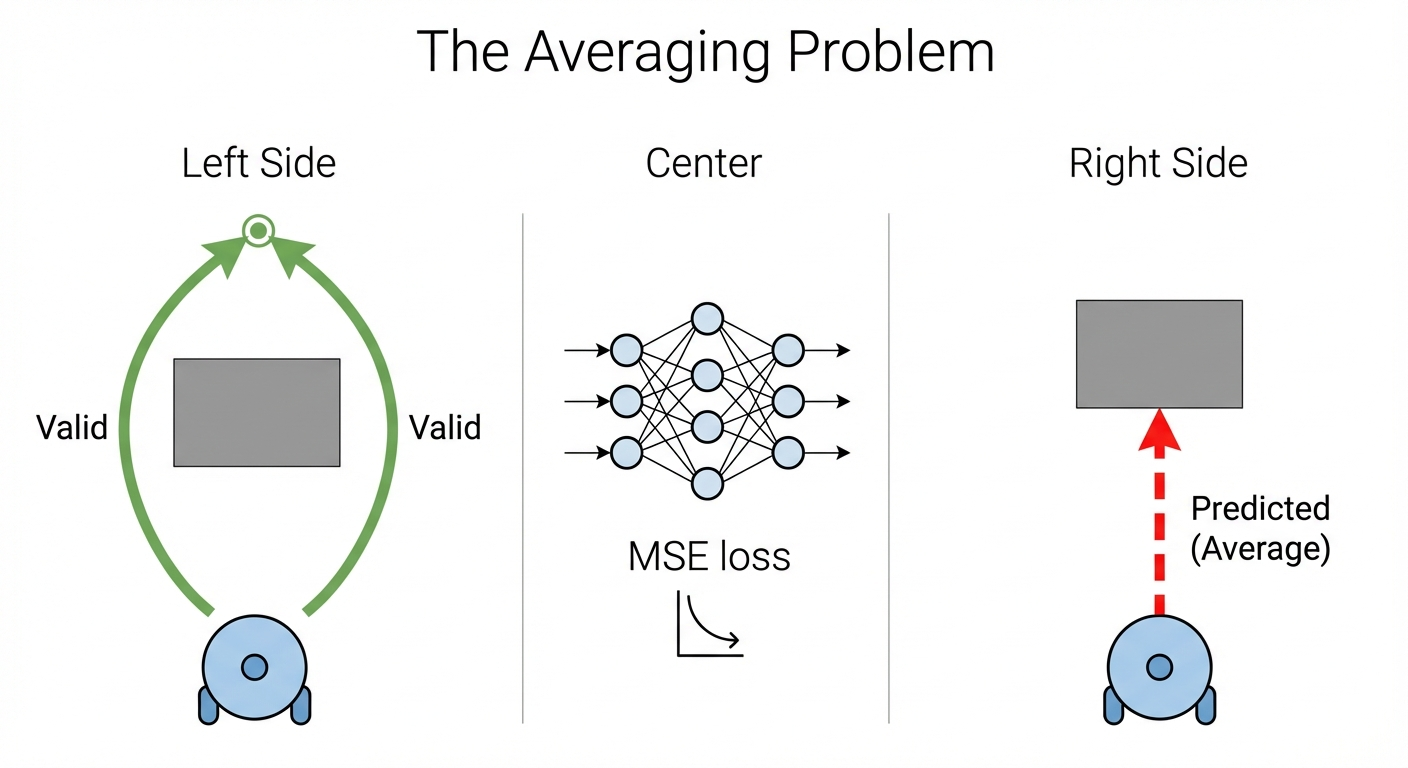
When demonstrations contain multiple valid actions for the same state, MSE loss produces the average of those actions. Going left and going right averages to going straight ahead — directly into the obstacle (Figure 2).
This isn’t a rare edge case. Multimodality appears everywhere in manipulation:
- Short-horizon: Approach an object from the left or right
- Long-horizon: Different orderings of subtasks (stack blocks A-B-C or C-B-A)
- Grasping: Multiple valid grasp poses for the same object
The mathematical reason is fundamental: neural networks with continuous activations draw smooth curves through data. They cannot represent the sharp discontinuity between “go left” and “go right” — the decision boundary would need to be infinitely steep.\(^{[2]}\)
What About Mixture Models?
You might think: “Use a Gaussian Mixture Model (GMM) to capture multiple modes!” Methods like LSTM-GMM try this, but face challenges:
- Must pre-specify the number of modes (how many valid actions exist?)
- Often biased toward one mode in practice
- Struggles with high-dimensional action spaces
These are still explicit policies — they output actions directly, just with a more flexible distribution.
Implicit Policies
Implicit policies take a different approach: instead of outputting actions directly, they learn an energy function \(E(s, a)\) over state-action pairs. Low energy = good action. This naturally represents multimodal distributions — multiple actions can have low energy.
Energy-based methods like Implicit BC (IBC)\(^{[3]}\) can represent arbitrary distributions, but require negative sampling during training — notoriously unstable and prone to mode collapse.
Enter Diffusion Policy
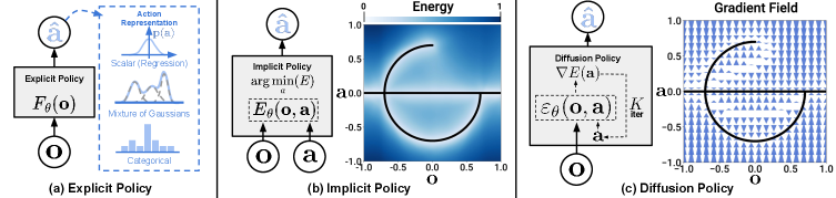
Here’s the key insight from Chi et al.\(^{[1]}\): diffusion models naturally represent multimodal distributions. The same property that lets them generate diverse images lets them generate diverse robot actions.
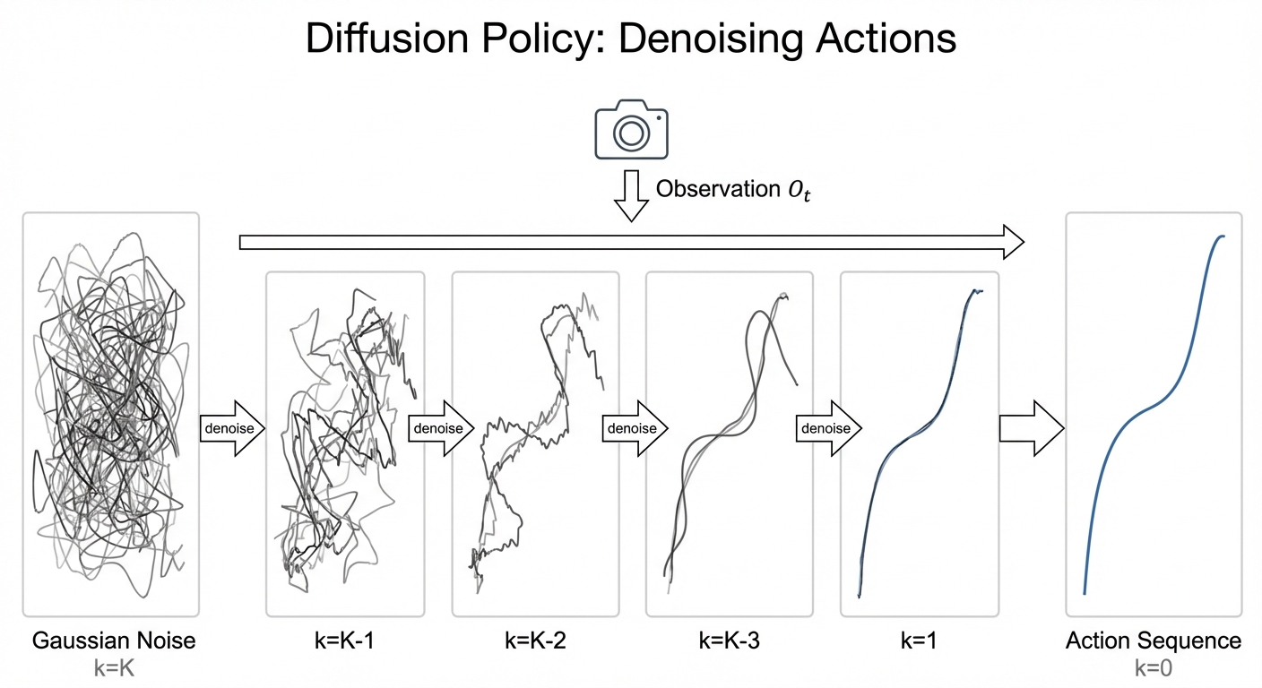
In image generation, diffusion starts with noise and iteratively refines it into a coherent image. For robotics, we start with noise and refine it into a coherent action sequence:
| Image Diffusion | Action Diffusion |
|---|---|
| Random pixels → Image | Random actions → Trajectory |
| Conditioned on text prompt | Conditioned on visual observation |
| Multiple valid images per prompt | Multiple valid trajectories per observation |
The denoising process acts like gradient descent on a learned energy landscape. Different random initializations converge to different modes — the policy “commits” to one valid action sequence per rollout while learning the full multimodal distribution.
Why Diffusion Handles Multimodality
Three mechanisms make this work:
Stochastic initialization: Each inference starts from random Gaussian noise, naturally exploring different modes
Score function learning: Instead of predicting actions directly, the network predicts the gradient of log-probability. This sidesteps the normalization constant that makes energy-based methods unstable
Iterative refinement: Langevin dynamics sampling follows the learned gradient field toward high-probability regions, allowing the model to express arbitrarily complex distributions
Langevin dynamics is a sampling algorithm that draws samples from a distribution using only its score function \(\nabla \log p(x)\):
\[ x_{t+1} = x_t + \frac{\eta}{2} \nabla \log p(x_t) + \sqrt{\eta} \, \epsilon, \quad \epsilon \sim \mathcal{N}(0, I) \]
Intuition: It’s gradient ascent with noise.
- The gradient term \(\nabla \log p(x)\) pushes toward high-probability regions
- The noise term \(\sqrt{\eta} \epsilon\) prevents getting stuck and enables exploration of multiple modes
Why it matters for diffusion: The reverse diffusion process is essentially Langevin dynamics with a time-varying score. The SDE formulation from Part 6 of our diffusion series shows this connection:
\[ dX_t = \underbrace{u_t^{target}}_{\text{deterministic flow}} + \underbrace{\frac{\sigma_t^2}{2} \nabla \log p_t}_{\text{score correction}} \, dt + \sigma_t \, dW_t \]
The score correction term is the Langevin-like component — it counteracts noise dispersion by pointing toward high-probability regions.
Watch this in action — Diffusion Policy learns both modes and commits to one per episode:
Diffusion Policy commits to one mode per rollout while learning multiple valid trajectories. Video from Chi et al.\(^{[1]}\)
Now let’s see exactly how this works mathematically.
The Diffusion Policy Formulation
Understanding the math is essential for debugging, tuning, and extending the method. Let’s make this precise. Given an observation \(O_t\), we want to sample from the action distribution \(p(A_t | O_t)\), where \(A_t\) is a sequence of future actions (more on this shortly).
Forward Process (Training)
During training, we gradually corrupt clean action sequences with noise. This teaches the network what noise “looks like” at each corruption level:
\[ A_t^k = \sqrt{\bar{\alpha}_k} \cdot A_t^0 + \sqrt{1 - \bar{\alpha}_k} \cdot \epsilon, \quad \epsilon \sim \mathcal{N}(0, I) \tag{2}\]
Here \(A_t^0\) is the clean action sequence from demonstrations, \(\epsilon\) is random Gaussian noise, \(k\) indexes diffusion timesteps (not robot timesteps), and \(\bar{\alpha}_k\) is a noise schedule controlling how much signal remains at step \(k\).
This paper uses DDPM (Ho et al. 2020), which is a discrete-time formulation. Our diffusion series uses a continuous-time SDE formulation (Song et al. 2021), which came later and simplified many things.
| DDPM (this paper, 2020) | Continuous SDE (our series, 2021+) | |
|---|---|---|
| Time | Discrete: \(k \in \{0, 1, ..., K\}\) | Continuous: \(t \in [0, 1]\) |
| Convention | \(k=0\) = data, \(k=K\) = noise | \(t=0\) = noise, \(t=1\) = data |
| Forward process | Markov chain with noise schedule \(\alpha_k, \beta_k\) | SDE: \(dX_t = f_t dt + g_t dW_t\) |
| Training | Variational lower bound derivation | Direct score matching |
| Noise schedule | Must carefully design \(\beta_1, ..., \beta_K\) | Simpler, often just linear |
Why continuous simplifies things:
- No complex schedules: DDPM requires careful tuning of discrete \(\beta_k\) values. Continuous formulation uses simpler schedules.
- Cleaner math: Theorems become equalities instead of bounds. The loss is tight, not a lower bound.
- Flexible sampling: Can use any number of steps at inference (10, 50, 100) without retraining.
The formulas:
| DDPM (discrete) | Continuous SDE (our series) |
|---|---|
| \(A^k = \sqrt{\bar{\alpha}_k} A^0 + \sqrt{1-\bar{\alpha}_k} \epsilon\) | \(dX_t = u_t(X_t) dt + \sigma_t dW_t\) |
| Forward: add noise step-by-step | Forward: continuous noising process |
| Reverse: predict \(\epsilon\), denoise | Reverse: follow score \(\nabla \log p_t\) |
The connection: DDPM is a discretization of the continuous VP-SDE. See Part 5 for the SDE derivation and Part 6 for score functions.
Reverse Process (Inference)
At test time, we start from pure noise and iteratively denoise (Figure 4):
\[ A_t^{k-1} = \frac{1}{\sqrt{\alpha_k}} \left( A_t^k - \frac{1 - \alpha_k}{\sqrt{1 - \bar{\alpha}_k}} \epsilon_\theta(O_t, A_t^k, k) \right) + \sigma_k z \tag{3}\]
Here \(\epsilon_\theta\) is a neural network predicting the noise, \(z \sim \mathcal{N}(0, I)\) is fresh noise for stochasticity, and \(\alpha_k, \sigma_k\) are schedule parameters. See the derivation below for how this formula arises.
The goal: We want to reverse the noising process. Given a noisy action, recover the clean one.
The key idea: If we knew what noise was added, we could subtract it out. We train a neural network to predict that noise.
Variables (refer back to these):
| Symbol | Meaning |
|---|---|
| \(A^0\) | Clean action (what we want) |
| \(A^k\) | Noisy action at diffusion step \(k\) |
| \(\epsilon\) | The actual noise that was added (unknown at inference) |
| \(\epsilon_\theta\) | Network’s prediction of the noise |
| \(\bar{\alpha}_k\) | Cumulative noise schedule (how much signal remains at step \(k\)) |
Step 1 — The forward process is a simple formula:
From Equation 2, we can write any noisy action as: \[A^k = \underbrace{\sqrt{\bar{\alpha}_k}}_{\text{signal scaling}} \cdot A^0 + \underbrace{\sqrt{1-\bar{\alpha}_k}}_{\text{noise scaling}} \cdot \epsilon\]
This is just: (scaled clean action) + (scaled noise). No iterative steps needed.
Step 2 — Rearrange to solve for the clean action:
If we knew the noise \(\epsilon\), we could solve for the clean action \(A^0\): \[A^0 = \frac{A^k - \sqrt{1-\bar{\alpha}_k} \cdot \epsilon}{\sqrt{\bar{\alpha}_k}}\]
Read this as: “subtract the scaled noise from the noisy action, then rescale.”
Step 3 — Train a network to predict the noise:
We don’t know the true noise \(\epsilon\) at inference time. So we train a neural network \(\epsilon_\theta\) to predict it from the noisy action and observation.
Substituting the network’s prediction gives us an estimate of the clean action: \[\hat{A}^0 = \frac{A^k - \sqrt{1-\bar{\alpha}_k} \cdot \epsilon_\theta(O, A^k, k)}{\sqrt{\bar{\alpha}_k}}\]
Step 4 — Use the estimate to take a denoising step:
We want \(p(A^{k-1} | A^k)\) — the reverse step. Using Bayes and conditioning on \(A^0\):
\[q(A^{k-1} | A^k, A^0) = \mathcal{N}(A^{k-1}; \tilde{\mu}_k, \tilde{\sigma}_k^2 I)\]
The posterior mean and variance work out to: \[ \tilde{\mu}_k = \frac{\sqrt{\bar{\alpha}_{k-1}} \beta_k}{1-\bar{\alpha}_k} A^0 + \frac{\sqrt{\alpha_k}(1-\bar{\alpha}_{k-1})}{1-\bar{\alpha}_k} A^k \] \[ \tilde{\sigma}_k^2 = \frac{\beta_k (1-\bar{\alpha}_{k-1})}{1-\bar{\alpha}_k} \]
where \(\beta_k = 1 - \alpha_k\) (noise added at step \(k\)).
Now substitute our estimate \(\hat{A}^0\) from Step 3. After simplification (grouping terms in \(A^k\) and \(\epsilon_\theta\)), we get Equation 3:
\[ A^{k-1} = \frac{1}{\sqrt{\alpha_k}} \left( A^k - \frac{1-\alpha_k}{\sqrt{1-\bar{\alpha}_k}} \epsilon_\theta \right) + \sigma_k z \]
The first term removes predicted noise; the second adds fresh noise for the next step.
Connection to our diffusion series:
In Part 6, we derived the conditional score function for a Gaussian. For DDPM’s forward process \(p_k(A^k | A^0) = \mathcal{N}(\sqrt{\bar{\alpha}_k} A^0, (1-\bar{\alpha}_k) I)\):
\[\nabla_{A^k} \log p_k(A^k | A^0) = -\frac{A^k - \sqrt{\bar{\alpha}_k} A^0}{1-\bar{\alpha}_k} = -\frac{\epsilon}{\sqrt{1-\bar{\alpha}_k}}\]
(The second equality uses the forward process: \(A^k - \sqrt{\bar{\alpha}_k} A^0 = \sqrt{1-\bar{\alpha}_k} \epsilon\))
Predicting noise is equivalent to predicting the score direction! The network learns which way leads to valid actions.
In Part 6, we also showed the SDE extension trick — given an ODE with drift \(u_t\), we can add noise while preserving the same probability path: \[dX_t = \left[u_t^{target} + \frac{\sigma_t^2}{2} \nabla \log p_t\right] dt + \sigma_t dW_t\]
The score term \(\frac{\sigma_t^2}{2} \nabla \log p_t\) corrects for noise dispersion, pointing samples toward high-probability regions. The DDPM reverse step is a discrete-time version of this principle.
The network \(\epsilon_\theta(O_t, A_t^k, k)\) learns to answer: “Given this noisy action sequence and this observation, what noise was added?”
Equivalently, it learns the score function — the gradient of log-probability pointing toward valid actions. The denoising process follows this gradient field from noise toward high-probability action sequences.
Training Objective
The training objective is beautifully simple. We add noise to expert actions, then train the network to predict what noise was added:
The loss is simply mean squared error between true and predicted noise:
\[ \mathcal{L}(\theta) = \mathbb{E}_{k, \epsilon, (A_t^0, O_t)} \left[ \| \epsilon - \epsilon_\theta(O_t, A_t^k, k) \|^2 \right] \tag{4}\]
This elegant formulation avoids the normalization constant entirely — we never need to compute \(Z = \int \exp(-E(a)) da\).
So far, we’ve focused on what to predict. But there’s another crucial design choice: predicting sequences of actions, not just single steps. This turns out to be just as important as the diffusion formulation itself.
Action Chunking: Predicting Sequences
A crucial design choice in Diffusion Policy is predicting sequences of future actions rather than single-step actions. This is called action chunking, and it solves several problems at once.
The Compounding Error Problem
In standard closed-loop control, errors compound quadratically:
With matched train/test distributions, total error scales as \(O(\epsilon T)\) — linear in horizon \(T\).
With distribution shift (the reality), error scales as \(O(\epsilon T^2)\) — quadratic growth.\(^{[4]}\)
A small mistake pushes the robot into unfamiliar states, causing larger mistakes, causing even more unfamiliar states…
Action chunking dramatically reduces this: a 500-step task with chunk size \(k=100\) becomes effectively a 5-step problem.
The Idle Action Problem
Human demonstrations contain pauses — waiting before prying open a lid, hesitating before a delicate insertion. A single-step policy sees the same observation and must choose between “stay still” and “move” — impossible from current state alone.
With action chunking, the sequence encodes timing implicitly: “stay still for 10 steps, then move.” The behavior becomes Markovian again as long as pauses fit within a chunk.
The Three Horizons
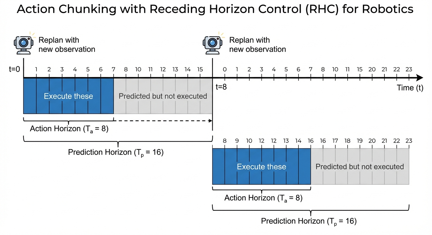
Diffusion Policy uses three temporal parameters (Figure 5):
| Parameter | Symbol | Typical Value | Description |
|---|---|---|---|
| Observation horizon | \(T_o\) | 2 | Past observation steps used as context |
| Prediction horizon | \(T_p\) | 16 | Future actions predicted by the model |
| Action horizon | \(T_a\) | 8 | Actions actually executed before replanning |
The key insight is \(T_a < T_p\): we predict more actions than we execute, then replan with updated observations.
Receding Horizon Control
This creates a receding horizon scheme:
Time 0: Predict actions [0, 1, 2, ..., 15]
        Execute actions [0, 1, 2, ..., 7]

Time 8: Observe new state
        Predict actions [8, 9, 10, ..., 23]
        Execute actions [8, 9, 10, ..., 15]

Time 16: Observe, replan, execute...Think of it like a GPS that continuously replans. You compute a route to the destination (prediction horizon), drive for a few miles (action horizon), then replan based on current position. This balances commitment to plans with responsiveness to new information.
Temporal ensembling further improves smoothness: query the policy at every timestep, producing overlapping predictions, then average them with exponential weights. This creates a voting mechanism across multiple predictions.\(^{[5]}\)
With the formulation and temporal structure established, what neural network architectures work best for learning the denoising function \(\epsilon_\theta\)?
Network Architectures
What neural network actually learns the denoising function \(\epsilon_\theta\)? The architecture choice significantly impacts both performance and training stability.
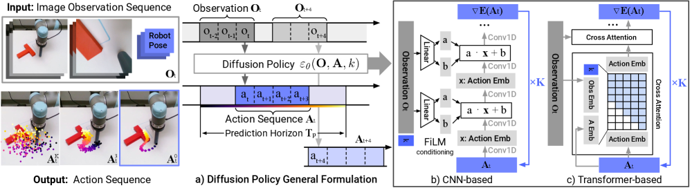
Diffusion Policy supports two architectures, each with distinct tradeoffs:
CNN-Based (U-Net)
The default architecture uses a 1D temporal U-Net (see Figure 6(b)):
- Visual encoder: ResNet-18 with spatial softmax pooling (extracts 32 keypoints per image)
- Denoising network: 1D convolutions along the time axis with FiLM conditioning
- Conditioning: Observations modulate every convolution layer via scale/shift
Strengths: Stable training, fewer hyperparameters, good default choice Weakness: Low-pass filtering bias — struggles with high-frequency action changes
Transformer-Based
The alternative uses a decoder-only transformer (see Figure 6(c)):
- Encoder: Processes conditioning (timestep embedding + observation embedding)
- Decoder: Generates action sequence with causal attention
- Cross-attention: Actions attend to observation embeddings in each layer
Strengths: Better for complex tasks, captures long-range dependencies Weakness: More hyperparameter-sensitive, requires careful tuning
Start with the CNN architecture (DP-C). It’s more stable and works well on most tasks. Switch to transformer (DP-T) if you see performance plateaus on complex, long-horizon tasks.
Visual Conditioning
Both architectures need to incorporate visual observations. A key design choice distinguishes Diffusion Policy from earlier diffusion-based planning methods: what distribution do we model?
Conditional vs. Joint Distributions
Diffusion Policy models the conditional distribution \(p(A_t | O_t)\) — actions given observations. This contrasts with Diffuser\(^{[7]}\) (Janner et al. 2022), which models the joint distribution \(p(A_t, O_t)\) over both actions and observations.
| Approach | What it models | How it generates actions |
|---|---|---|
| Diffuser (joint \(p(A, O)\)) | Actions and future states together | Denoise both actions and predicted future observations |
| Diffusion Policy (conditional \(p(A \| O)\)) | Actions given observations | Denoise only actions, observations are fixed inputs |
Diffuser generates trajectories — sequences of (action, state) pairs. It must predict what will happen in the world. Diffusion Policy generates only actions — it doesn’t predict future states, just reacts to current observations.
From the paper:
“This formulation allows the model to predict actions conditioned on observations without the cost of inferring future states, speeding up the diffusion process and improving the accuracy of generated actions.”
The practical benefits:
No state prediction errors: Diffuser must accurately predict future observations to plan through them. Errors compound. Diffusion Policy sidesteps this entirely — it never predicts what the world will look like.
Faster inference: Denoising a 16-step action sequence is faster than denoising a 16-step trajectory of (action, observation) pairs. The exclusion of observation features from the denoising output “significantly improves inference speed and better accommodates real-time control.”
More accurate actions: The network capacity focuses entirely on action quality, not split between action and state prediction.
Why Conditional Modeling Works
You might wonder: is directly conditioning on observations theoretically valid? Don’t we need to model the full joint distribution to capture dependencies?
The answer comes from how conditional diffusion training works (see Guidance in our diffusion series). The key insight:
When training conditional diffusion, the noise target \(\epsilon\) doesn’t depend on the conditioning variable \(O_t\): \[ u_t^{target}(A_t^k | A_t^0, O_t) = u_t^{target}(A_t^k | A_t^0) \]
Why? Because the forward process (adding noise to actions) is purely mechanical — it doesn’t care about observations. The noise schedule corrupts actions the same way regardless of what the robot saw.
This means we can train the conditional model \(p(A|O)\) with the same loss as unconditional diffusion — we just include \(O_t\) as an additional network input:
\[ \mathcal{L}(\theta) = \mathbb{E}_{k, \epsilon, (A_t^0, O_t)} \left[ \| \epsilon - \epsilon_\theta(O_t, A_t^k, k) \|^2 \right] \]
The network learns to denoise actions given observations. By sampling \((A_t^0, O_t)\) pairs from demonstration data and regressing against the noise \(\epsilon\), least-squares regression automatically learns the conditional distribution — no joint modeling required.
This is identical to how text-to-image diffusion works: Stable Diffusion models \(p(\text{image} | \text{text})\), not \(p(\text{image}, \text{text})\). The conditioning (text prompt) enters through cross-attention, and the model learns to generate images that match the prompt without ever modeling the joint distribution of images and text.
Efficient Feature Extraction
A practical benefit of conditional modeling: observations are extracted once per inference, not once per denoising step.
- Extract visual features from images
- Run 10-100 denoising iterations using those same features
- Total visual encoding cost: 1x, not 10-100x
For FiLM conditioning (CNN architecture), the observation modulates the denoising network at every layer:
The idea: Instead of concatenating the observation to the input (which only affects the first layer), we let the observation modulate every layer of the network.
The mechanism: For each hidden layer with features \(h\):
\[ h' = \gamma(O_t, k) \odot h + \beta(O_t, k) \tag{5}\]
| Symbol | Meaning |
|---|---|
| \(h\) | Hidden features from the denoising network (e.g., 256-dim vector) |
| \(\gamma\) | Scale parameters — “how much to amplify each feature” |
| \(\beta\) | Shift parameters — “what baseline to add to each feature” |
| \(\odot\) | Element-wise multiplication |
| \(O_t, k\) | The observation and diffusion timestep |
Intuition: A small network takes \((O_t, k)\) and outputs \(\gamma\) and \(\beta\) vectors. These act like “dials” that adjust how the main network processes information:
- \(\gamma\) controls which features matter — amplify task-relevant features, suppress irrelevant ones
- \(\beta\) controls the baseline — shift feature activations based on context
Example: If the observation shows “gripper is near the cup”, FiLM might amplify features related to grasping and suppress features related to navigation.
Why it works: This is more expressive than simple concatenation. The observation can influence how the network computes, not just what it computes on.
One remaining challenge: the iterative denoising is slow. If we need 100 steps per action prediction, that’s too slow for real-time robotics.
DDIM: Fast Inference
Standard DDPM requires as many denoising steps as training noise levels (typically 100). This is too slow for real-time control.
DDIM (Denoising Diffusion Implicit Models)\(^{[6]}\) decouples training and inference:
- Training: 100 noise levels
- Inference: 10 denoising steps
- Result: ~0.1 second latency on an NVIDIA 3080
Why Can We Skip Steps?
This seems suspicious: we trained the network to denoise step-by-step, so how can we skip 90% of steps at inference?
DDPM training teaches the network to predict the noise \(\epsilon\) added at each step — not just “how to go from step \(k\) to step \(k-1\)”.
This noise prediction implicitly encodes the direction toward the clean data: \[ \hat{A}^0 = \frac{A^k - \sqrt{1-\bar{\alpha}_k} \cdot \epsilon_\theta(A^k, k)}{\sqrt{\bar{\alpha}_k}} \]
From any noisy point \(A^k\), we can directly estimate the clean action \(\hat{A}^0\).
DDIM exploits this: instead of taking tiny steps, it jumps directly toward the predicted clean point, then adds back the appropriate noise level for the target step.
The full DDIM update formula (equation 12 from the paper) has three components:
\[ A^{k-1} = \underbrace{\sqrt{\bar{\alpha}_{k-1}} \cdot \hat{A}^0}_{\text{(1) predicted clean}} + \underbrace{\sqrt{1-\bar{\alpha}_{k-1} - \sigma_k^2} \cdot \epsilon_\theta}_{\text{(2) direction to } A^k} + \underbrace{\sigma_k \epsilon}_{\text{(3) noise}} \]
where \(\hat{A}^0 = \frac{A^k - \sqrt{1-\bar{\alpha}_k} \cdot \epsilon_\theta}{\sqrt{\bar{\alpha}_k}}\) is the predicted clean action.
| Component | What it does |
|---|---|
| (1) Predicted clean | Where we think the clean data is, scaled to target noise level |
| (2) Direction to \(A^k\) | Points back toward current noisy sample — preserves consistency |
| (3) Random noise | Optional stochasticity (σ=0 for deterministic DDIM) |
For deterministic DDIM (σ=0, what Diffusion Policy uses):
\[ A^{k'} = \sqrt{\bar{\alpha}_{k'}} \cdot \hat{A}^0 + \sqrt{1-\bar{\alpha}_{k'}} \cdot \epsilon_\theta \]
Step-by-step what happens:
- Start at \(A^{100}\) (pure noise)
- Predict noise \(\epsilon_\theta(A^{100}, 100)\)
- Compute predicted clean: \(\hat{A}^0 = \frac{A^{100} - \sqrt{1-\bar{\alpha}_{100}} \cdot \epsilon_\theta}{\sqrt{\bar{\alpha}_{100}}}\)
- Jump to intermediate level \(A^{90}\) using the formula above
- From \(A^{90}\), predict noise again → get a better \(\hat{A}^0\)
- Jump to \(A^{80}\), repeat…
Why can’t we just output \(\hat{A}^0\) directly?
Because the noise prediction \(\epsilon_\theta\) is imperfect. The network makes errors, and these errors are amplified when we directly invert the formula.
| Noise level | Signal-to-noise | Prediction quality |
|---|---|---|
| \(k=100\) (mostly noise) | Low | Poor — hard to see the clean data |
| \(k=50\) (mixed) | Medium | Better — more signal to work with |
| \(k=10\) (mostly clean) | High | Good — easy to predict small noise |
The iterative refinement helps because:
- Each step moves to a lower noise level where predictions are more accurate
- Errors from step \(k\) get corrected at step \(k-1\)
- It’s like GPS: walk partway, get a new reading (more accurate now), adjust course
Can we do one-step generation?
Yes, but it requires special training:
- Consistency Models\(^{[9]}\) train the network to map ANY noise level directly to \(A^0\)
- Progressive Distillation trains a student network to match a multi-step teacher in fewer steps
These methods achieve 1-4 step generation but need extra training. Standard DDPM/DDIM networks aren’t optimized for single-step accuracy.
Intuition: GPS vs. Turn-by-Turn
Think of navigation:
DDPM is like turn-by-turn directions: “In 100 meters, turn left. In 50 meters, turn right…” You must follow every instruction.
DDIM is like having GPS coordinates: you know the destination, so you can take larger steps (highways) while still ending at the same place.
The network’s noise prediction acts as “destination coordinates” — it points toward clean data regardless of the current noise level.
Why It Works Theoretically
DDIM defines a non-Markovian diffusion process that has the same marginal distributions as DDPM at each timestep \(t\), but allows deterministic jumps between any two timesteps.
The mathematics: DDPM’s forward process is: \[ A^k = \sqrt{\bar{\alpha}_k} A^0 + \sqrt{1 - \bar{\alpha}_k} \epsilon \]
This is a closed-form expression — we can jump directly from \(A^0\) to any \(A^k\) without intermediate steps. DDIM simply inverts this relationship, using the network’s noise estimate to reconstruct the trajectory.
Fewer steps = faster but noisier. Diffusion Policy uses 10 inference steps (10× speedup) with minimal quality loss. For robotics, this trade-off is worthwhile: real-time control matters more than perfect trajectory smoothness.
You might ask: if we can infer with 10 steps, why train with 100?
Key clarification: Training with “100 noise levels” does NOT mean running 100 sequential steps per training example. Instead:
- Sample a random noise level \(k \sim \text{Uniform}(1, 100)\)
- Add noise at that level: \(A^k = \sqrt{\bar{\alpha}_k} A^0 + \sqrt{1-\bar{\alpha}_k} \epsilon\)
- Train the network to predict \(\epsilon\)
Each training batch sees a random mix of noise levels. The network learns to denoise at ALL corruption levels — from barely noisy (\(k=1\)) to pure noise (\(k=100\)).
Can you train with fewer levels? Yes! Recent work shows this is task-dependent:
| Task Type | Optimal Training Steps | Why |
|---|---|---|
| Refinement (denoising, super-resolution) | 10-100 | Small changes need few corruption levels |
| Conditional generation (Diffusion Policy) | 100 | Moderate complexity |
| Unconditional image generation | 1000 | Must learn full data distribution |
Fast-DDPM\(^{[8]}\) showed that for medical image-to-image tasks (a form of conditional generation), 10 training steps can actually outperform more — additional steps hurt quality because the “convergence area” (late timesteps) provides diminishing returns. While robotics differs from medical imaging, the principle applies: conditional generation needs fewer steps than unconditional.
The key asymmetry: Training samples noise levels in parallel (cheap), inference runs steps sequentially (expensive). So even if you train with many levels, you want to infer with few.
For robotics: Diffusion Policy uses 100 training steps — a reasonable middle ground for conditional action generation. This is much less than the 1000 steps typical for image generation.
This enables 10Hz real-time control — fast enough for most manipulation tasks.
Results
We’ve covered the theory: multimodality problem, diffusion solution, action chunking, architectures, and fast inference. But does it actually work? It was evaluated on 12 tasks across 4 benchmarks:
Simulation Results
| Task | Diffusion Policy | Best Baseline | Improvement |
|---|---|---|---|
| Push-T | 95% | 20% (LSTM-GMM) | +75% |
| Block Push (4 blocks) | 84% | 28% (BET) | +56% |
| ToolHang | 89% | 73% (LSTM-GMM) | +16% |
| Transport | 94% | 90% (LSTM-GMM) | +4% |
Average improvement: 46.9% across all tasks.
Real-World Results
On physical robots (UR5, Franka):
| Task | Success Rate |
|---|---|
| Push-T (UR5) | 95% |
| Mug Flipping | 90% |
| Sauce Pouring | 0.74 IoU (vs 0.79 human) |
The Push-T Visualization
The Push-T task beautifully demonstrates multimodal learning. The robot must push a T-shaped block to a target pose — approachable from left or right.
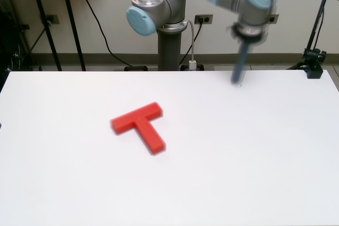
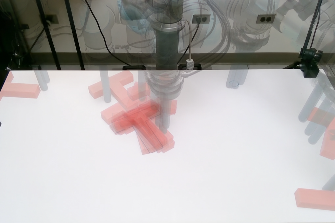
The difference is striking (Figure 7):
- LSTM-GMM (Figure 7 (b)): Biased toward one approach, gets stuck
- IBC: Fails to commit, produces jittery motion
- BET: Indecisive, oscillates between modes
- Diffusion Policy (Figure 7 (a)): Learns both modes, commits to one per episode
Robustness to Perturbations
The policy also handles unexpected disturbances gracefully — occlusion, perturbation during pushing, and interference during the finish:
Diffusion Policy recovers from hand occlusion (0:05) and physical perturbation (0:11, 0:39). Video from Chi et al.\(^{[1]}\)
Common Misconceptions
Given these strong results, you might wonder what the catch is. Let’s address the most common concerns:
With DDIM, inference takes ~100ms — fast enough for 10Hz control. The Consistency Policy further reduces this to single-step generation via distillation.
Diffusion Policy achieves strong results with 50-200 demonstrations. The action chunking reduces effective horizon, and diffusion’s inductive biases help generalization.
Counterintuitively, position control outperforms velocity control for Diffusion Policy. Why?
- Absolute positions are easier to denoise than relative velocities — the network learns “where to be” rather than “how fast to move”
- Built-in error correction: If the robot drifts, the next position target corrects it automatically
- Velocity control compounds errors: Small prediction errors accumulate over time
- Robustness to latency: Position targets remain valid even with control delays
You might wonder: don’t motors need velocity/torque commands to move? How can a policy output just positions?
The answer is the control hierarchy:
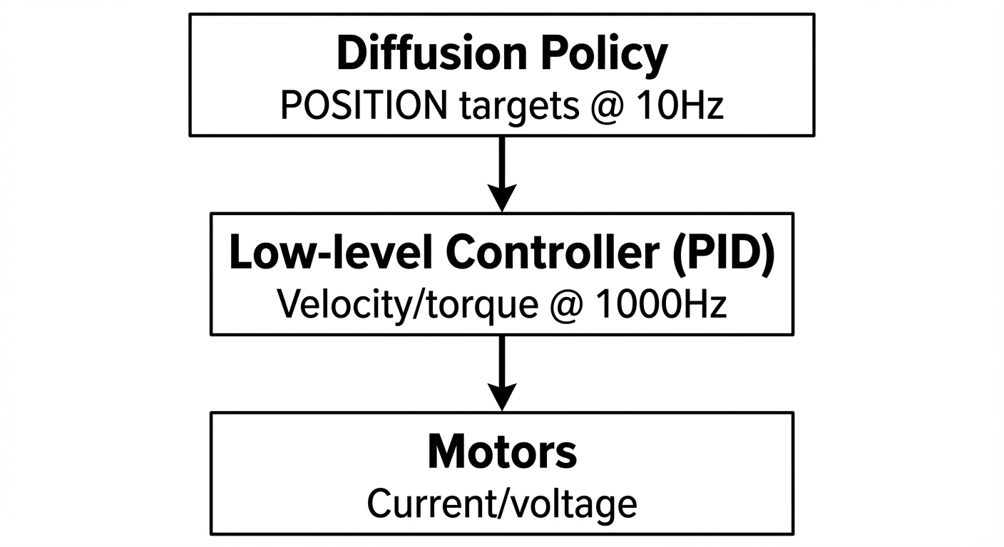
The robot’s built-in PID controller handles the position → velocity conversion:
\[ \text{velocity} = K_p \cdot (\text{target} - \text{current}) + K_d \cdot \frac{d(\text{error})}{dt} \]
This runs at ~1000Hz internally — much faster than the policy’s 10Hz outputs.
Analogy: It’s the difference between:
- Velocity control: “Turn steering wheel 15° left for 2 seconds” — if timing is off, you crash
- Position control: “Drive to GPS coordinates (37.77, -122.42)” — the car continuously corrects toward target
The low-level controller is “free” — it’s already on the robot. The policy just says where to go, not how.
“Position control” can mean two different things:
| Representation | What it specifies | Example |
|---|---|---|
| Joint positions | Angle of each motor | [θ₁, θ₂, θ₃, θ₄, θ₅, θ₆, θ₇] |
| End-effector pose | Gripper location + orientation | [x, y, z, roll, pitch, yaw] |
Diffusion Policy uses joint positions — and so do ACT, ALOHA, and π₀.
Why not end-effector? If you specify gripper position (x, y, z), the robot must solve inverse kinematics (IK) to find joint angles:
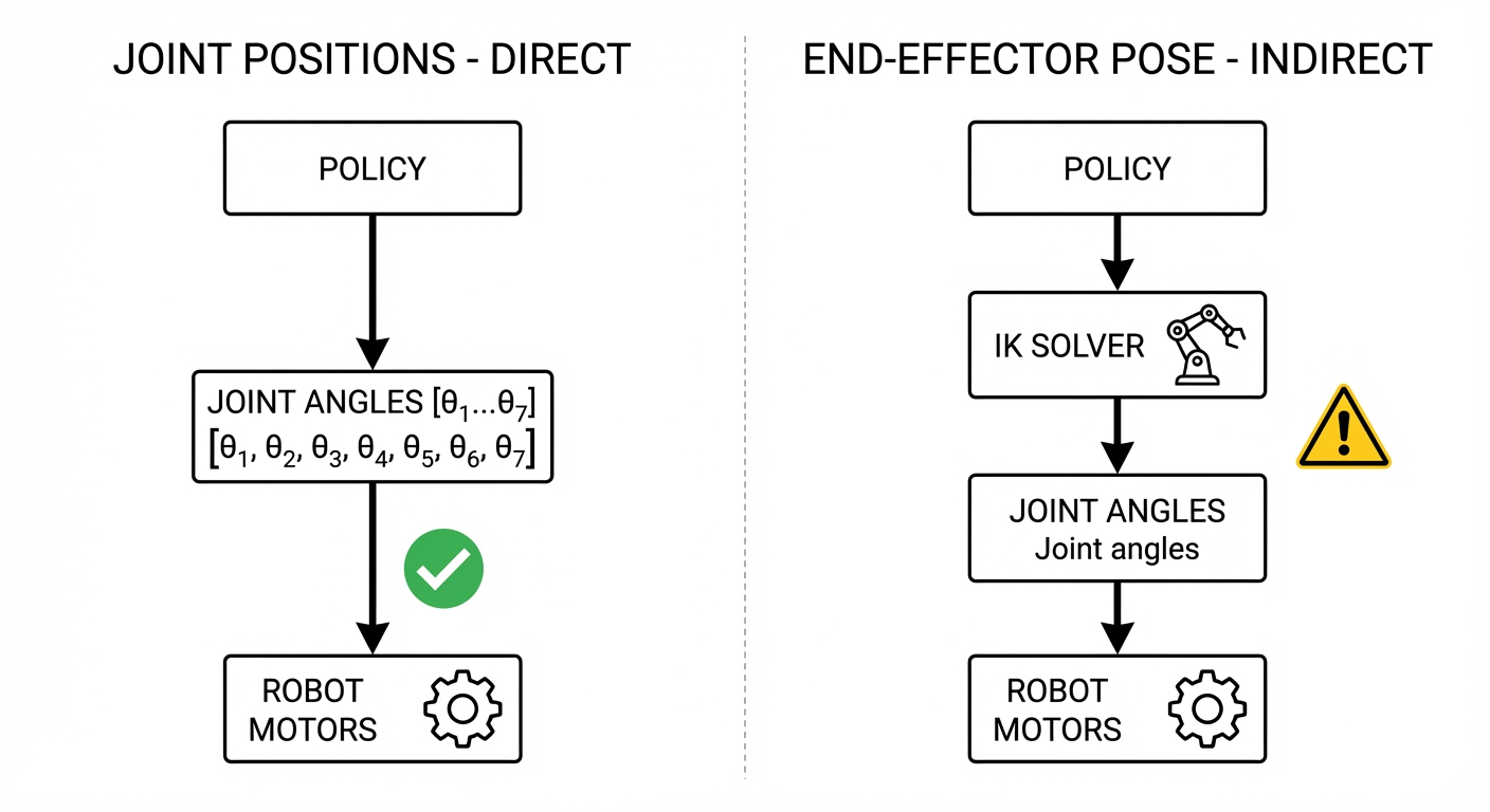
IK is problematic because:
- Non-unique: Multiple joint configurations reach the same point (elbow up vs down)
- Can fail: Near singularities or workspace boundaries
- Adds latency: Extra computation between policy and robot
Why some papers still use end-effector:
- Cross-robot transfer: Different arms have different joints, but all have a gripper at
(x, y, z) - Easier demonstrations: Humans think in “move gripper here”, not joint angles
| Joint positions | End-effector pose | |
|---|---|---|
| Precision | ✅ Direct | ⚠️ IK errors |
| Cross-robot | ❌ Robot-specific | ✅ Generalizes |
| Demos | ⚠️ Need joint recording | ✅ Natural teleoperation |
The field has split into two camps:
| Approach | Papers | Control Mode | Trade-off |
|---|---|---|---|
| Joint positions | ACT, ALOHA, π₀, GR00T N1 | Absolute positions | High precision, single embodiment |
| Delta end-effector | RT-1, RT-2, OpenVLA, Octo | Relative deltas | Cross-robot transfer |
Key finding: Papers focused on precision manipulation (ACT, ALOHA, π₀) use absolute joint positions — validating Diffusion Policy’s insight. Papers focused on cross-embodiment transfer (RT-X, OpenVLA) use delta end-effector because it generalizes across different robot arms.
Both camps adopted action chunking to reduce compounding errors — which provides similar benefits to position control.
Connection to Optimal Control Theory
The empirical results are impressive, but why does diffusion work so well? Here’s a surprising theoretical result: for simple systems, diffusion policy provably recovers the optimal controller.
The Setup
Consider the simplest possible robotics scenario:
- Linear dynamics: \(s_{t+1} = As_t + Ba_t + w_t\) where \(w_t \sim \mathcal{N}(0, \Sigma_w)\)
- Expert uses linear feedback: \(a_t = -Ks_t\) (e.g., from solving an LQR problem)
Here \(s_t\) is the state, \(a_t\) is the action, and \(K\) is the optimal feedback gain matrix.
The Result
When you train a diffusion policy on demonstrations from this expert, the optimal denoiser converges to:
\[ \epsilon_\theta(s, a, k) = \frac{1}{\sigma_k}(a + Ks) \]
At inference time, DDIM sampling finds the global minimum at \(a = -Ks\) — exactly the optimal control law!
The diffusion policy doesn’t just imitate actions. It recovers the underlying control structure.
Intuition: What’s Happening?
Think about what the denoiser is doing:
- During training: It sees state-action pairs \((s, a)\) where \(a = -Ks + \text{noise}\)
- It learns: The “noise” relative to the clean action is \((a - (-Ks)) = a + Ks\)
- At inference: Starting from random noise, DDIM iteratively removes this “error”, converging to \(a = -Ks\)
The diffusion process is essentially learning: “given this state, what’s the residual between noisy and optimal action?”
Multi-Step Extension
For trajectory prediction (\(T_p > 1\)), diffusion learns to predict:
\[ a_{t+t'} = -K(A - BK)^{t'} s_t \]
This is exactly what you’d get from rolling out the optimal controller! The policy implicitly learns the task-relevant dynamics model \((A - BK)\) needed to predict future optimal actions.
This analysis shows diffusion isn’t just “memorizing demonstrations” — it’s learning the structure of optimal control. For linear systems, this is provable. For nonlinear robotic tasks, empirical results suggest similar structure-learning happens.
This may explain why diffusion generalizes well: it captures the underlying control law, not just surface-level action patterns.
Who’s Using This?
This theoretical grounding helps explain why Diffusion Policy has become the foundation for robot learning research:
- Physical Intelligence (π₀): Their flagship robot policy uses diffusion for action generation
- Google DeepMind: Incorporated diffusion into several manipulation systems
- Stanford Mobile ALOHA: Uses diffusion for bimanual mobile manipulation
- NVIDIA Isaac Lab: Supports diffusion policy training out of the box
If you hear “diffusion for robotics” in 2024-2025, it almost certainly traces back to this paper.
Practical Implementation
If you want to try Diffusion Policy yourself:
LeRobot: Hugging Face’s LeRobot library includes Diffusion Policy with pretrained weights
Official Implementation: The original codebase includes all benchmarks
Simulation First: Start with Push-T in simulation before moving to real hardware
From the paper’s recommended settings:
- Observation horizon: \(T_o = 2\)
- Prediction horizon: \(T_p = 16\)
- Action horizon: \(T_a = 8\)
- Training diffusion steps: 100
- Inference diffusion steps: 10 (DDIM)
- Batch size: 256
- Learning rate: 1e-4 with cosine decay
Open Questions and Recent Progress
If you want to try it yourself, the code is available and well-documented. But the original Diffusion Policy paper left several open questions. Here’s what we know now (as of early 2026):
1. “Diffusion is Too Slow” — Solved ✅
| Method | Year | Inference Time | Speedup |
|---|---|---|---|
| Diffusion Policy | 2023 | ~1000ms | 1x |
| Consistency Policy | 2024 | ~100ms | 10x |
| OneDP | 2024 | 16ms (62Hz) | 40x |
| LightDP | 2025 | 2.7ms | 93x |
Key techniques: Consistency distillation, model pruning, streaming approaches. LightDP achieves <10ms on mobile hardware (iPhone 13).
2. “Can’t Scale to Humanoids” — Solved ✅
| System | DoF | Key Innovation |
|---|---|---|
| iDP3 on Fourier GR1 | 25 | Egocentric 3D diffusion, no calibration |
| Boston Dynamics Atlas | 50 | 450M param DiT, flow-matching, 30Hz control |
| RDT-1B | 14+ | 1.2B params, 46 datasets |
Boston Dynamics + Toyota Research Institute deployed a 450M parameter Diffusion Transformer controlling the full Atlas humanoid for industrial tasks (rope tying, tire manipulation).
3. Optimal Action Chunk Length — Task-Dependent ⚠️
No universal answer. Research findings:
| Task Type | Optimal Chunk | Why |
|---|---|---|
| Long-horizon manipulation | 8-16 steps | Balances consistency and replanning |
| High-precision contact | 1-4 steps | Needs fast reactive feedback |
| Bimanual coordination | 50-100 steps | Requires temporal coherence |
Key insight: Control-theoretic analysis shows action chunking provides stability guarantees by circumventing exponential error compounding — but longer isn’t always better.
Adaptive methods now exist: BID selects optimal chunks at test-time, Real-Time Chunking enables smooth execution for VLAs.
4. Why Does Diffusion Actually Work? — Surprising Answer 🤔
The most interesting recent finding from Simchowitz et al. (2025):
Diffusion policies do NOT owe their success primarily to capturing multimodality or expressing complex distributions.
The actual mechanism: iterative computation with supervised intermediate steps.
A simple two-step regression policy (MIP) matches flow-based policy performance on most benchmarks.
This suggests the “diffusion” framing may be less important than: - Multiple refinement steps (iterative computation) - Intermediate supervision during training - Appropriate stochasticity for exploration
5. Nonlinear Control Theory — Active Research 📚
The linear LQR result from the paper has been extended:
- Elamvazhuthi et al. (2024): For control-affine systems, diffusion can exactly track trajectories when Lie bracket controllability conditions hold
- S2Diff (2025): Lyapunov-guided diffusion provides stability guarantees via the “Almost Lyapunov theorem”
- DIAL-MPC (2024): MPPI is equivalent to a single-stage diffusion process — connecting sampling-based MPC to score functions
Open question: Can we characterize exactly what “structure” diffusion learns for general nonlinear tasks?
Research Insights
Beyond the technical contributions and open problems, this paper offers deeper lessons for researchers:
The Real Contribution Isn’t “Diffusion for Robotics”
The surface-level reading is “we applied diffusion to robot actions.” The actual insight is deeper: the choice of action distribution representation fundamentally limits what a policy can learn.
Before this paper, people tried to fix multimodality with more data, bigger networks, or clever losses. This paper says: the problem is architectural — Gaussian outputs can’t represent multimodal distributions, period. No amount of training fixes that.
Challenging Dogma Leads to Insight
The position control finding is counterintuitive. For years, robotics assumed velocity/delta control was better because it’s “local” and doesn’t compound errors. This paper shows the opposite — for learned policies with observation noise, position control wins.
Why? Because learned policies aren’t perfect. Given imperfect predictions, position control provides free error correction via the low-level controller.
Broader lesson: Optimal design for perfect systems differs from optimal design for learned systems with errors. Question assumptions that were derived for classical (non-learned) settings.
The Right Factorization Depends on the Task
The choice to model \(p(A|O)\) instead of \(p(A, O)\) is a statement about what the robot needs to know:
- Diffuser models the joint \(p(A, O)\) because it’s doing planning — predicting what will happen
- Diffusion Policy models the conditional \(p(A|O)\) because it’s doing reaction — trusting observations to arrive
Research direction: Hybrid approaches might use different factorizations at different horizons — plan long-term (joint), react short-term (conditional).
Action Chunking Connects to Temporal Abstraction
Predicting 16 actions instead of 1 isn’t just about smoothness — it’s a form of temporal abstraction. This connects to:
- Options framework in RL (Sutton et al.)
- Motor primitives in neuroscience
- Hierarchical planning in classical robotics
Research direction: Maybe the right abstraction for robot learning isn’t actions or trajectories, but “motion sketches” — intent without over-specification.
The Meta-Lesson: Import and Adapt
The biggest insight is methodological: import successful techniques from adjacent fields and carefully adapt them.
Diffusion worked for images because images are high-dimensional and multimodal. Robot actions share these properties. The adaptation (conditional modeling, action chunks, position control) required domain knowledge, but the core insight transferred.
Research strategy: When stuck, ask “what other field solved a structurally similar problem?”
What’s Next?
Diffusion Policy works. But it has a limitation: you need to train a separate policy for every task.
What if you could tell a robot “pick up the red cup” in natural language — and it just does it? No task-specific training. No reward engineering.
That’s where Vision-Language-Action (VLA) models come in. They combine the language understanding of GPT-4 with the action generation of Diffusion Policy. The result: robots that learn from the internet and follow arbitrary instructions.
In Part 2, we’ll explore how π0, OpenVLA, and other VLAs are creating the first generalist robot policies — and why 2024-2026 is shaping up to be robotics’ “GPT moment.”
We’ve seen why naive behavioral cloning fails — averaging multimodal actions produces nonsense — and how Diffusion Policy solves this by representing actions as a denoising process. The key innovations are:
- Diffusion for actions: Start from noise, iteratively refine into valid trajectories
- Action chunking: Predict sequences to reduce compounding errors and capture temporal dependencies
- Receding horizon: Balance commitment with responsiveness by replanning frequently
- Efficient conditioning: Extract visual features once, reuse across denoising steps
The result is a 46.9% average improvement over prior methods, with strong real-world performance on manipulation tasks.
The framework is surprisingly simple once you see it: replace the image output of a diffusion model with action sequences, condition on observations instead of text, and apply standard denoising. The elegance lies in how naturally diffusion handles the multimodality that makes robot learning hard.
Push-T comparison figures (Figure 7) from the Diffusion Policy project page, used with attribution.
References
[1] Chi, C., Feng, S., Du, Y., Xu, Z., Cousineau, E., Burchfiel, B., & Song, S. Diffusion Policy: Visuomotor Policy Learning via Action Diffusion. RSS 2023, IJRR 2024. Project page
[2] Decisiveness in Imitation Learning for Robots. Google Research Blog, 2023.
[3] Florence, P., Lynch, C., Zeng, A., Ramirez, O., Wahid, A., Downs, L., Wong, A., Lee, J., Mordatch, I., & Tompson, J. Implicit Behavioral Cloning. CoRL 2021.
[4] Ross, S., Gordon, G., & Bagnell, D. A Reduction of Imitation Learning and Structured Prediction to No-Regret Online Learning. AISTATS 2011.
[5] Zhao, T., Kumar, V., Levine, S., & Finn, C. Learning Fine-Grained Bimanual Manipulation with Low-Cost Hardware. RSS 2023. (ACT paper)
[6] Song, J., Meng, C., & Ermon, S. Denoising Diffusion Implicit Models. ICLR 2021.
[7] Janner, M., Du, Y., Tenenbaum, J., & Levine, S. Planning with Diffusion for Flexible Behavior Synthesis. ICML 2022. (Diffuser)
[8] Jiang, Z., et al. Fast-DDPM: Fast Denoising Diffusion Probabilistic Models for Medical Image-to-Image Generation. arXiv 2024. (Shows 10 training steps can outperform 100 for refinement tasks)
[9] Song, Y., et al. Consistency Models. ICML 2023. (One-step generation via distillation)
Further Reading
- Diving into Diffusion Policy with LeRobot — Excellent code walkthrough
- Diffusion Policy Project Page — Official demos and code
- diffusion-literature-for-robotics — Curated paper list