Categories of Inference-Time Scaling for Improved LLM Reasoning
Subtitle: And an Overview of Recent Inference-Scaling Papers (Including Recursive Language Models)
Date: JUL 19, 2025
URL: https://magazine.sebastianraschka.com/p/categories-of-inference-time-scaling
Image Count: 17
Images

Figure - Caption: The State of LLM Reasoning Model Inference
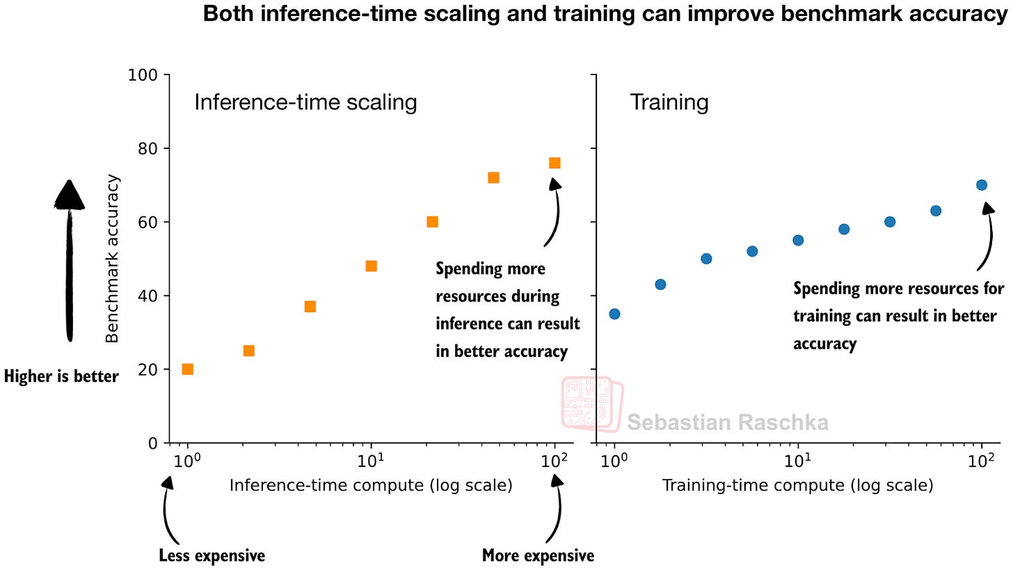
Figure - Caption: Figure 1: Spending additional resources during inference (left) and training (right) generally improves the model’s accuracy.
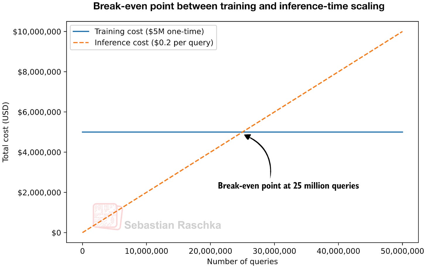
Figure - Caption: Figure 2: Given some assumptions where training adds a specific upfront cost and inference scaling adds no upfront cost but makes each query more expensive, we can find a break-even point.
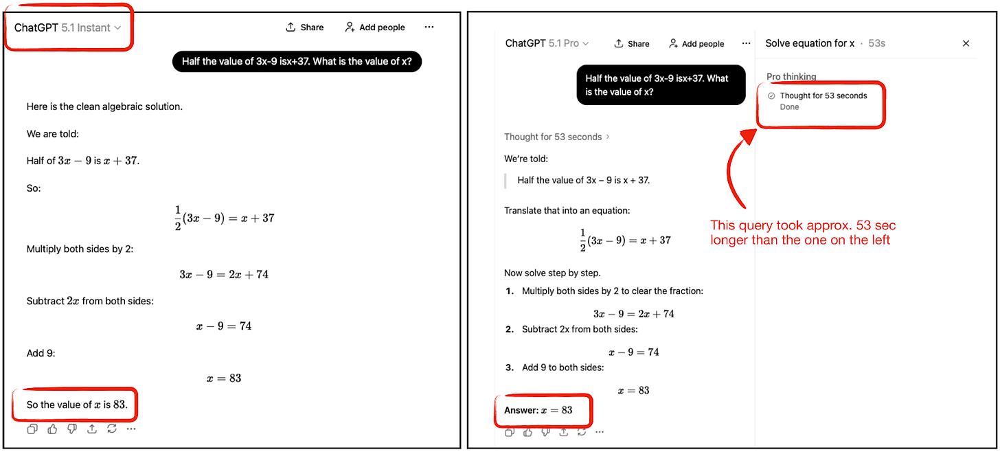
Figure - Caption: Figure 3: Example using an “Instant” model with minimal inference scaling and using GPT-5.1 Pro, which uses an enormous amount of inference scaling.
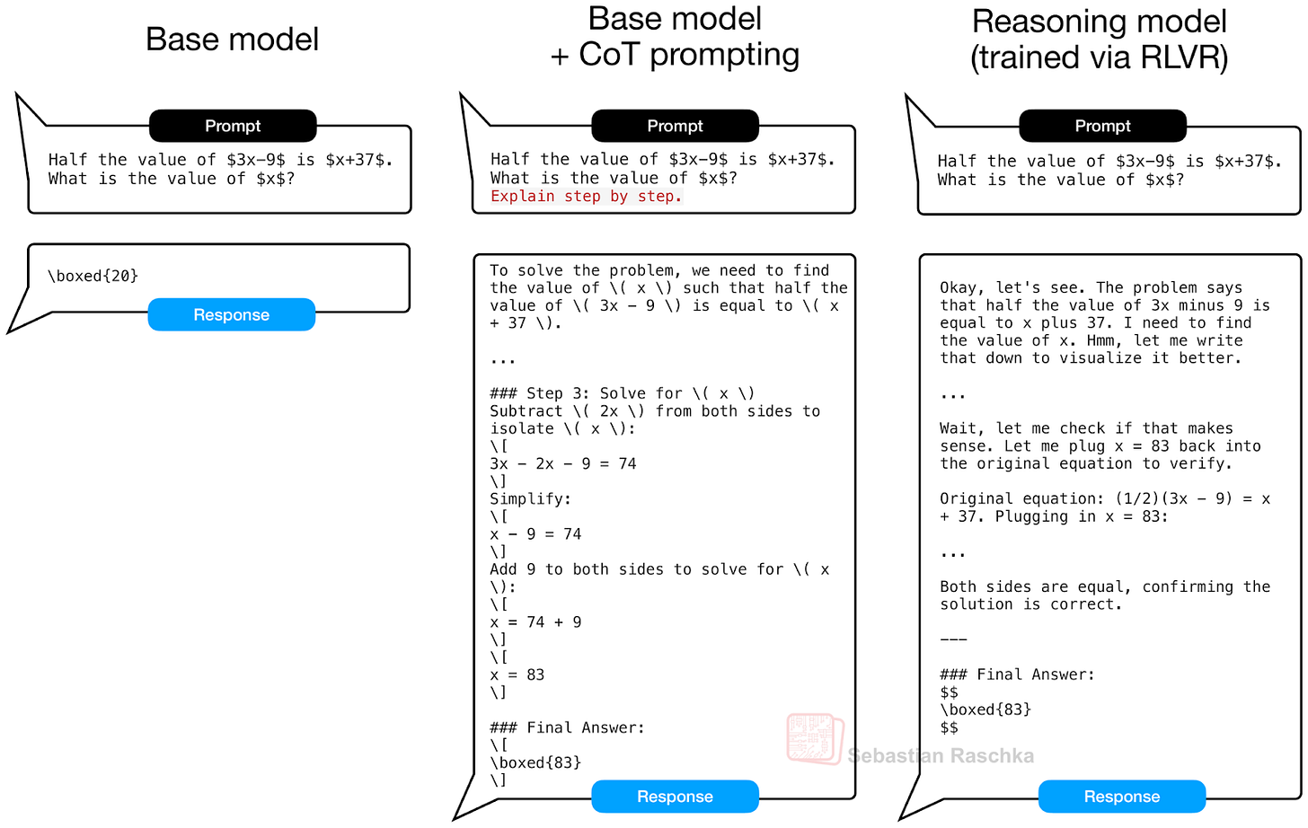
Figure - Caption: Figure 4: Real outputs via Qwen3 0.6B base and reasoning model on a MATH-500 test set query. When using CoT prompting, the base model explains the answer more often (center), similar to the reasoning model, which can improve the answer accuracy.
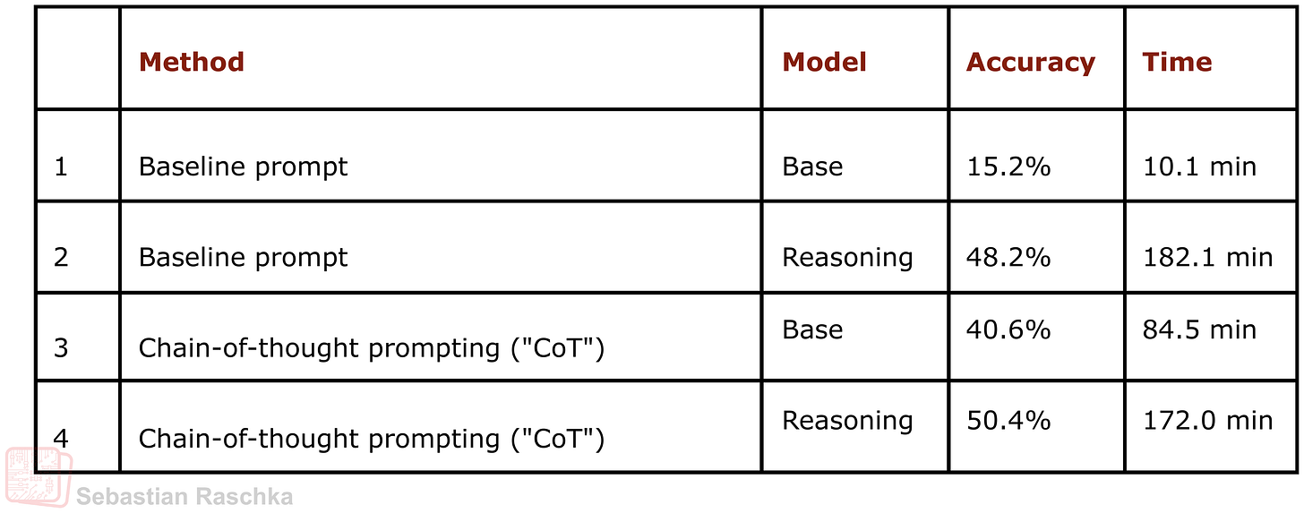
Figure - Caption: Figure 5: Chain-of-thought prompting vs no chain-of-thought prompting on 500 math questions from MATH-500. The base model accuracy benefits substantially, but it also increases the runtime substantially since more tokens are produced for each of the answers.
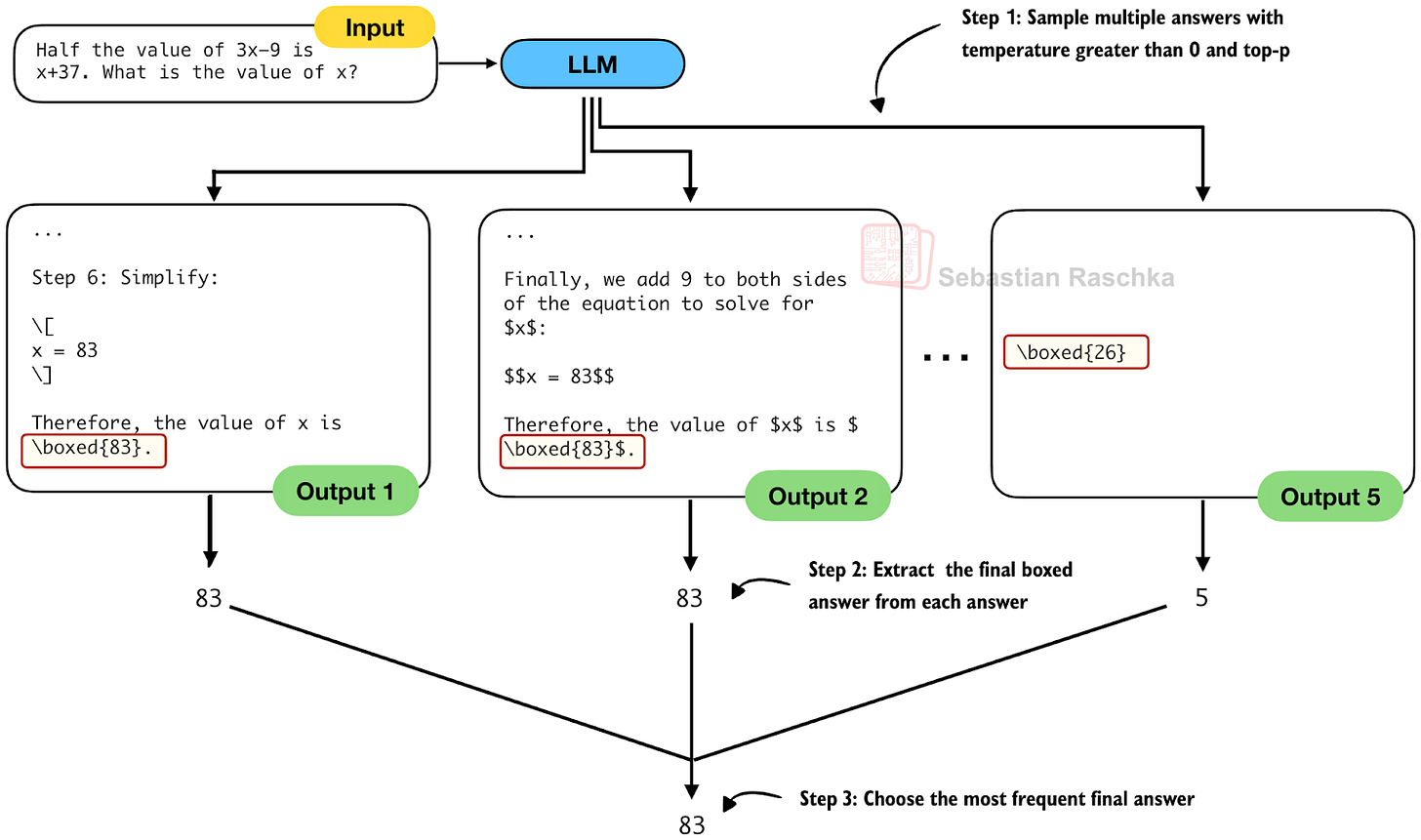
Figure - Caption: Figure 6: An illustration of self-consistency sampling.
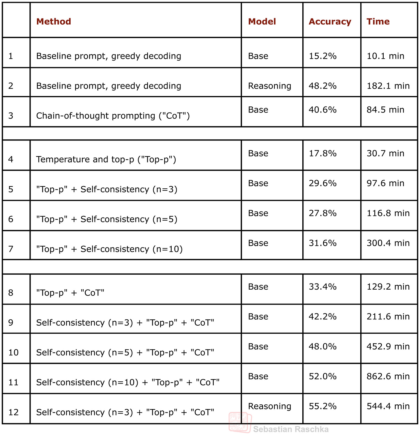
Figure - Caption: Figure 7: This table shows MATH-500 task accuracy for different inference-scaling methods. The experiments were run on a DGX Spark in a single-sample sequential (as opposed to batched and/or parallel) mode. You can find the code to reproduce these results here on GitHub.
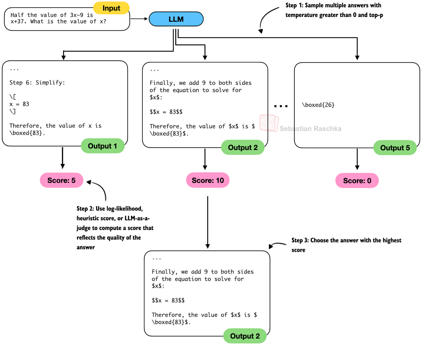
Figure - Caption: Figure 8: An illustration of Best-of-N ranking.
Figure
- Caption: Figure 9: An illustration of rejection sampling.
Figure
- Caption: Figure 10: An illustration of self-refinement.

Figure
- Caption: Figure 11: An illustration of Tree-of-Thoughts sampling.
Figure
- Caption: Annotated figure from the RLM paper, https://arxiv.org/abs/2512.24601
Figure
- Caption: Annotated figure from the RLM paper, https://arxiv.org/abs/2512.24601
Figure
- Caption: Figure 12: An excerpt of an earlier table showing the performance of the baselines without inference scaling (rows 1 and 2) and several flavors of self-consistency (rows 9-12).
Figure
- Caption: Figure 13: Figure from the DeepSeekMath-V2 report showing how the answer improves with an increasing number of self-refinement iterations.
Figure
- Caption: Excerpt of chapter 4 in Build a Reasoning Model (From Scratch)
Full Text Content
Inference scaling has become one of the most effective ways to improve answer quality and accuracy in deployed LLMs.
The idea is straightforward. If we are willing to spend a bit more compute, and more time at inference time (when we use the model to generate text), we can get the model to produce better answers.
Every major LLM provider relies on some flavor of inference-time scaling today. And the academic literature around these methods has grown a lot, too.
Back in March, I wrote an overview of the inference scaling landscape and summarized some of the early techniques.
The State of LLM Reasoning Model Inference SEBASTIAN RASCHKA, PHD · MARCH 8, 2025 Read full story
In this article, I want to take that earlier discussion a step further, group the different approaches into clearer categories, and highlight the newest work that has appeared over the past few months.
As part of drafting a full book chapter on inference scaling for Build a Reasoning Model (From Scratch), I ended up experimenting with many of the fundamental flavors of these methods myself. With hyperparameter tuning, this quickly turned into thousands of runs and a lot of thought and work to figure out which approaches should be covered in more detail in the chapter itself. (The chapter grew so much that I eventually split it into two, and both are now available in the early access program.)
PS: I am especially happy with how the chapter(s) turned out. It takes the base model from about 15 percent to around 52 percent accuracy, which makes it one of the most rewarding pieces of the book so far.
What follows here is a collection of ideas, notes, and papers that did not quite fit into the final chapter narrative but are still worth sharing.
I also plan to add more code implementations to the bonus materials on GitHub over time.
Table of Contents (Overview)
Inference-Time Scaling Overview
Chain-of-Thought Prompting
Self-Consistency
Best-of-N Ranking
Rejection Sampling with a Verifier
Self-Refinement
Search Over Solution Paths
Conclusions, Categories, and Combinations
Bonus: What Do Proprietary LLMs Use?
You can use the left-hand navigation bar in the article’s web view to jump directly to any section.
- Inference-Time Scaling Overview
Inference-time scaling (also called inference-compute scaling, test-time scaling, or just inference scaling) is an umbrella term for methods that allocate more compute and time during inference to improve model performance.
This idea has been around for a long time, and one can think of ensemble methods in classic machine learning as an early example of inference-time scaling. I.e., using multiple models requires more compute resources but can give better results.
Even in LLM contexts, this idea has been around for a long time. However, I remember it became particularly popular (again) when OpenAI showed an inference-time scaling and training plot in one of their o1 announcement blog articles last year (Learning to Reason with LLMs).
Figure 1: Spending additional resources during inference (left) and training (right) generally improves the model’s accuracy.
I think this figure, adapted from OpenAI’s blog post, nicely captures the idea behind the two knobs we can use to improve LLMs. We can spend more resources during training (more data, bigger models, more or longer training stages) or inference.
Actually, in practice, it’s even better to do both at the same time: train a stronger model and use additional inference scaling to make it even better.
In this article, I only focus on the left part of the figure, inference-time scaling techniques, i.e., those training-free techniques that don’t change the model weights.
1.1 Training or Inference-Time Scaling: Which One Offers the Better Bang for the Buck?
I often get asked: what should we focus on, (more) training or inference scaling.
Training is usually very, very expensive, but it is a one-time cost. Inference-scaling is comparatively cheap, but it’s a cost we pay at each query.
Below is an illustration using napkin math with a lot of assumptions to illustrate the main point in a brief manner.
Let’s assume we have an LLM (or an LLM-powered application) that we want to improve by 5% on a given benchmark or problem and do a simple thought experiment. Additionally, let’s assume:
We don’t pass the extra cost for this improvement down to the customer.
We could either train the LLM longer for $5 million to achieve the same 5% improvement.
Or, for the same 5% improvement, we could pay $0.2 extra per query due to higher token usage.
What strategy is better for our company? If we had to choose between the two, then it really depends on how many queries you (or the users) plan to run for the lifetime of that LLM.
In this case, the break-even point is 5,000,000 dollars / 0.20 dollars per query = 25 million queries.
Figure 2: Given some assumptions where training adds a specific upfront cost and inference scaling adds no upfront cost but makes each query more expensive, we can find a break-even point.
For example, if each user runs 10 queries per day on average, we reach 25 million queries with about 25,000,000 / (10 per day) = 2.5 million user-days, which is roughly 7,000 daily active users for one year. If we have fewer than 7,000 daily users, or fewer than 10 queries per user on average, and plan to replace the LLM in about a year, then training is not worth it.
Pro tip: YPro tip: You don’t need to choose between the two. We can do both, more training and inference scaling to get a >5% improvement :).
1.2 Latency Requirements
In the example above, we looked at cost. However, time is another aspect to consider. Training adds a high upfront cost, and if we have to deploy a model next week, it could be a blocker.
Inference-time scaling adds a smaller upfront cost, in terms of implementing, trying, and comparing different methods. However, it adds a (depending on the technique, sometimes non-trivial) latency to each query. If we have strict latency requirements, for example, doubling the latency may be non-negotiable.
Figure 3: Example using an “Instant” model with minimal inference scaling and using GPT-5.1 Pro, which uses an enormous amount of inference scaling.
In the example shown in the figure above, the GPT-5.1 Pro version using more inference scaling took 53 seconds longer to prepare the answer (both models answered correctly, and while additional inference scaling tends to improve the answer accuracy as a whole, it can be wasteful for simple queries and add more latency.)
However, we also have to distinguish between sequential and parallel inference-scaling techniques (while GPT-5.1 Pro may involve parallel techniques as well, the additional runtime was almost certainly largely owed to a sequential technique). Given sufficient compute hardware, parallel inference scaling techniques can keep the runtime almost constant.
All in all, there are many practical considerations that need to be explored and addressed on a project-specific basis. In the following sections, my goal is to provide an overview of the different inference-scaling techniques that are interesting, popular, and often used today.
- Chain-of-Thought Prompting
Chain-of-thought (CoT) prompting is perhaps the prototypical example of inference scaling. Around the time when the Let’s Verify Step by Step paper was shared in 2023, we all experimented with prompt modifications like “Let’s verify step by step”, “Explain step by step”, and so on, as it made the model not only explain its answer but also sometimes improve the accuracy of that answer.
Figure 4: Real outputs via Qwen3 0.6B base and reasoning model on a MATH-500 test set query. When using CoT prompting, the base model explains the answer more often (center), similar to the reasoning model, which can improve the answer accuracy.
CoT prompting becomes unnecessary if your model already naturally explains its answer. E.g., models trained via Reinforcement Learning with Verifiable Rewards (like DeepSeek R1, Kimi K2 Thinking, and many others) generate these explanations automatically. (This can be a blessing and a curse, since this tends to yield better answers but also makes the model much more expensive to run due to the large amount of tokens it generates.)
However, when working with a base model, CoT prompting is basically a very useful trick to emit explanations. It doesn’t provide the model with new knowledge, but it makes the model use its knowledge better. Below are some of the results showing that adding CoT prompting can indeed be useful for a base model (but not so much for the reasoning model, as expected). The results below are for the MATH-500 test set.
Figure 5: Chain-of-thought prompting vs no chain-of-thought prompting on 500 math questions from MATH-500. The base model accuracy benefits substantially, but it also increases the runtime substantially since more tokens are produced for each of the answers.
(You can reproduce the results above via the cot_prompting_math500.py script. The runtimes are for a simple, sequential, uncompiled run through the MATH-500 test set using a DGX Spark. You can speed up the process by using the batched script and the –compile flag.)
If you are experimenting with a base model, it makes a lot of sense to combine CoT prompting with any of the other techniques described in the next sections. If your model already emits reasoning-chain-like explanations, CoT prompting is unnecessary.
Besides the original flavor of CoT prompting explained above, there are also many newer flavors of CoT prompting. The list below contains a few of the newer interesting 2025 papers that fall into this category.
2.1 Chain-of-Thought Papers (2025)
Below is a list of papers related to chain-of-thought (CoT) prompting. Note that the list is not exhaustive, and I also only focus on 2025 papers from my bookmark list.
31 Jan 2025, s1: Simple Test-Time Scaling, https://arxiv.org/abs/2501.19393
Here, researchers implement a budget-forcing mechanism that appends “Wait” tokens to prompt the model to emit longer reasoning chains (and truncates it when a given budget is reached).
30 May 2025, AlphaOne: Reasoning Models Thinking Slow and Fast at Test Time, https://arxiv.org/abs/2505.24863
This work is essentially a modification of the s1 method discussed above. They define an “α-moment” (”aha”-moment) that expands the thinking budget, then stochastically insert “wait” tokens before that point to trigger slow reasoning (where slow reasoning means generating more tokens to expand the answer). They then finally force a shift into fast reasoning (i.e., generating short, very direct responses) by converting later “wait” tokens into “”. This so-called “slow-then-fast” schedule improves accuracy across math, coding, and science tasks.
25 Feb 2025, Chain of Draft: Thinking Faster by Writing Less, https://arxiv.org/abs/2502.18600
This method works similarly to CoT prompting, but it aims to reduce the length of the intermediate reasoning chain by focusing more on minimalist intermediate drafting (like we humans do, for instance, when we scribble down intermediate steps when working on a math problem).
10 Feb 2025, ReasonFlux: Hierarchical LLM Reasoning via Scaling Thought Templates, https://arxiv.org/abs/2502.06772
Where CoT shifts the model into a “reasoning mode,” this ReasonFlux method shifts the model into a “template-guided reasoning mode.” I.e., it uses different types of prompt templates based on the problem to elicit reasoning. (Caveat: It’s not a pure inference-scaling method as it does require training the model to use these structured templates.)
8 Jan 2025, Towards System 2 Reasoning in LLMs: Learning How to Think With Meta Chain-of-Thought, https://arxiv.org/abs/2501.04682
Meta-CoT is an extension of CoT “by explicitly modeling the underlying reasoning required to arrive at a particular CoT”.
This is again a method that requires some additional training before it can be applied as an inference scaling method.
How it works is that after training, the model does not just emit a linear CoT, but it emulates the latent search process that underlies it. This means exploring branches, backtracking, and verifying intermediate states, etc., before committing to a final solution.
I am grouping it here as an extension of CoT, but I could also have added it to either the self-refine or tree-of-thought categories below. In this case, the grouping is not clear-cut. We can roughly think of the different methods as
CoT = one path
Tree-of-thought = many paths explored externally (outside the model’s forward path)
Meta-CoT = many paths explored internally.
- Self-Consistency
Self‑consistency, as described in Self-Consistency Improves Chain-of-Thought Reasoning in Language Models (2022), sounds like a fancy technique, but it simply has the model generate multiple answers (via temperature scaling and sampling). It then selects the answer that appears most often via majority vote.
Figure 6: An illustration of self-consistency sampling.
In short, self-consistency is essentially a form of ensembling (but with a single model and temperature sampling) and majority vote.
The higher the number of samples, the larger the compute requirements. And, up to a saturation point, larger samples improve accuracy.
This method is very simple on the surface, but it performs incredibly well, even in 2025, for example, as the recent Think Deep, Think Fast: Investigating Efficiency of Verifier-free Inference-time-scaling Methods (2025) paper discussed:
For reasoning models, majority voting proves to be a robust inference strategy, generally competitive or outperforming other more sophisticated inference-time-compute methods like best-of-N and sequential revisions, while the additional inference compute offers minimal improvements.
Another big advantage of this method is that it can be easily parallelized, since each answer can be generated independently (either via batching or across different devices).
For base models, it makes sense to combine this method with CoT prompting from the previous section. The table below compares the self-consistency approach with different sample sizes to the baseline without sampling, as well as consistency sampling combined with CoT prompting.
Figure 7: This table shows MATH-500 task accuracy for different inference-scaling methods. The experiments were run on a DGX Spark in a single-sample sequential (as opposed to batched and/or parallel) mode. You can find the code to reproduce these results here on GitHub.
Based on the results in the table above, in the case of Qwen3 0.6B and MATH-500 benchmark, it seems that self-consistency with a sample size of 3 already gives relatively good results (row 9 vs row 8). We can further improve accuracy with sample sizes 5 and 10, but this increases the runtime substantially. (However, note that the sampling can be further parallelized, which is not done here.)
You can find the code to reproduce these results here on GitHub.
3.1 Self-Consistency Papers (2025)
18 Apr Think Deep, Think Fast: Investigating Efficiency of Verifier-free Inference-time-scaling Methods, https://arxiv.org/abs/2504.14047
This paper doesn’t introduce a new method, but it provides a nice, comprehensive comparison of existing methods. Interestingly, it finds that self-consistency with majority voting (as opposed to any more sophisticated method involving reranking with a verifier) performs really well. This is consistent with my observations as well. Self-consistency with majority voting is a baseline that’s hard to beat.
23 May 2025, First Finish Search: Efficient Test-Time Scaling in Large Language Models, https://arxiv.org/abs/2505.18149
In this paper, the authors leverage the observation that reasoning tasks with shorter traces are much more likely to be correct than those with longer ones, as well as the fact that self-consistency can be efficiently parallelized across multiple devices, since each query runs independently.
So, here, the idea is that they launch n generation processes, and return as soon as one completes. That’s it.
21 May, Learning to Reason via Mixture-of-Thought for Logical Reasoning, https://arxiv.org/abs/2505.15817
At first glance, MoT looks superficially similar to self-consistency because the final answer comes from multiple reasoning traces and may be determined by majority vote (or a scoring method). However, unlike regular self-consistency, they aim to sample multiple reasoning modalities. E.g., … ,
1 Dec, The Art of Scaling Test-Time Compute for Large Language Models, https://arxiv.org/abs/2512.02008
This paper takes a systematic look at inference-time scaling strategies and evaluates them across eight modern LLMs (7B to 235B), including reasoning models (DeepSeek-R1, DAPO-32B, QwQ-32B, Qwen3-32B, GPT-OSS-120B) and non-reasoning models (DeepSeek-Chat, Qwen3-235B).
The conclusion is that there is no universally best inference-scaling strategy. The optimal choice depends on the model’s reasoning abilities, compute budget, and (surprisingly) not the difficulty of the problem.
Self-consistency (here called “majority voting”) performs surprisingly well, though.
- Best-of-N Ranking
Best-of-N ranking (or just Best-of-N) is a method very similar to self-consistency, which we discussed in the previous section. The main difference is that Best-of-N uses a scoring method to determine the best answer(s) rather than using a majority vote. The scoring method can be anything from log‑likelihood to heuristic scores to a learned verifier (LLM-as-a-judge).
Figure 8: An illustration of Best-of-N ranking.
In these cases, self-consistency doesn’t make sense, but Best-of-N remains applicable because it selects candidates based on a scoring function rather than on how often the same short answer appears.
In Best-of-N, we (can) still generate multiple samples in parallel, like in self-consistency, but then use, for example, an LLM (or some sort of heuristic) score (rank), and select the best answer.
The disadvantage of Best-of-N is that it tends to do worse than self-consistency in domains where self-consistency is applicable.
This claim is based on my personal experience, but there is also a new study, Think Deep, Think Fast: Investigating Efficiency of Verifier-free Inference-time-scaling Methods (2025), that found:
For reasoning models, simpler strategies such as majority voting often surpass more intricate methods like best-of-N or sequential revisions in performance.
4.1 Best-of-N Papers (2025)
25 Feb, Scalable Best-of-N Selection for Large Language Models via Self-Certainty, https://arxiv.org/abs/2502.18581
The method uses the model’s own token-level probability distributions to estimate how confident it is in each sampled response. They call this metric self-certainty, defined as how far the predicted token distribution deviates from a uniform one.
On the surface, this looks like classic log-likelihood scoring of the model’s own answers. However, classic log-likelihood scoring evaluates only the probabilities of the tokens that were actually sampled. Their self-certainty method scores the entire probability distribution over all tokens at every step. (They penalize distributions that are flat and reward distributions that are sharp.)
18 Apr Think Deep, Think Fast: Investigating Efficiency of Verifier-free Inference-time-scaling Methods, https://arxiv.org/abs/2504.14047
I already listed the paper under self-consistency, but I am also adding it again here for completeness (for those who skipped the previous section).
This paper doesn’t introduce a new method, but it’s a nice and comprehensive comparison of existing methods. Interestingly, it finds that self-consistency with majority voting (as opposed to any more sophisticated method involving reranking with a verifier) performs really well. This is consistent with my observations as well. Self-consistency with majority voting is a baseline that’s hard to beat.
18 Feb, Evaluation of Best-of-N Sampling Strategies for Language Model Alignment, https://arxiv.org/abs/2502.12668
This method still samples many outputs, as with regular Best-of-N. But instead of picking the top score, it adjusts the score with a regularization penalty. Specifically, (1) it penalizes answers that diverge too much from the base model’s normal style. Then, it adds another penalty (2) to prefer answers that are semantically consistent with the rest of the samples.
17 Apr 2025, Heimdall: Test-Time Scaling on the Generative Verification, https://arxiv.org/abs/2504.10337
This work introduces a verifier-centric form of Best-of-N scaling. Instead of sampling many solutions and picking the best one directly, Heimdall repeatedly samples the verification chains to judge correctness.
Interestingly, the paper shows that verification accuracy (the correctness of the verification) itself follows a strong scaling curve.
So, by combining multiple solver outputs with multiple verification passes, the method selects the answer with the highest pessimistic confidence (i.e., selecting the most likely correct solution with the least uncertainty). We can think of this as effectively combining Best-of-N over solutions with Best-of-N over verifier trajectories.
22 Jan 2025, Test-Time Preference Optimization (TPO): On-the-Fly Alignment via Iterative Textual Feedback, https://arxiv.org/abs/2501.12895
This work proposes a preference-driven form of Best-of-N. Or, alternatively, we can think of it as self-refinement enhanced with multiple samples, as in Best-of-N. Instead of only sampling many candidates and choosing the highest-scoring one, this method introduces an iterative refinement loop guided by a reward model. Each iteration samples several responses, scores them, compares the best and worst, and turns that comparison into textual critiques that the model then uses to rewrite its answer.
- Rejection Sampling with a Verifier
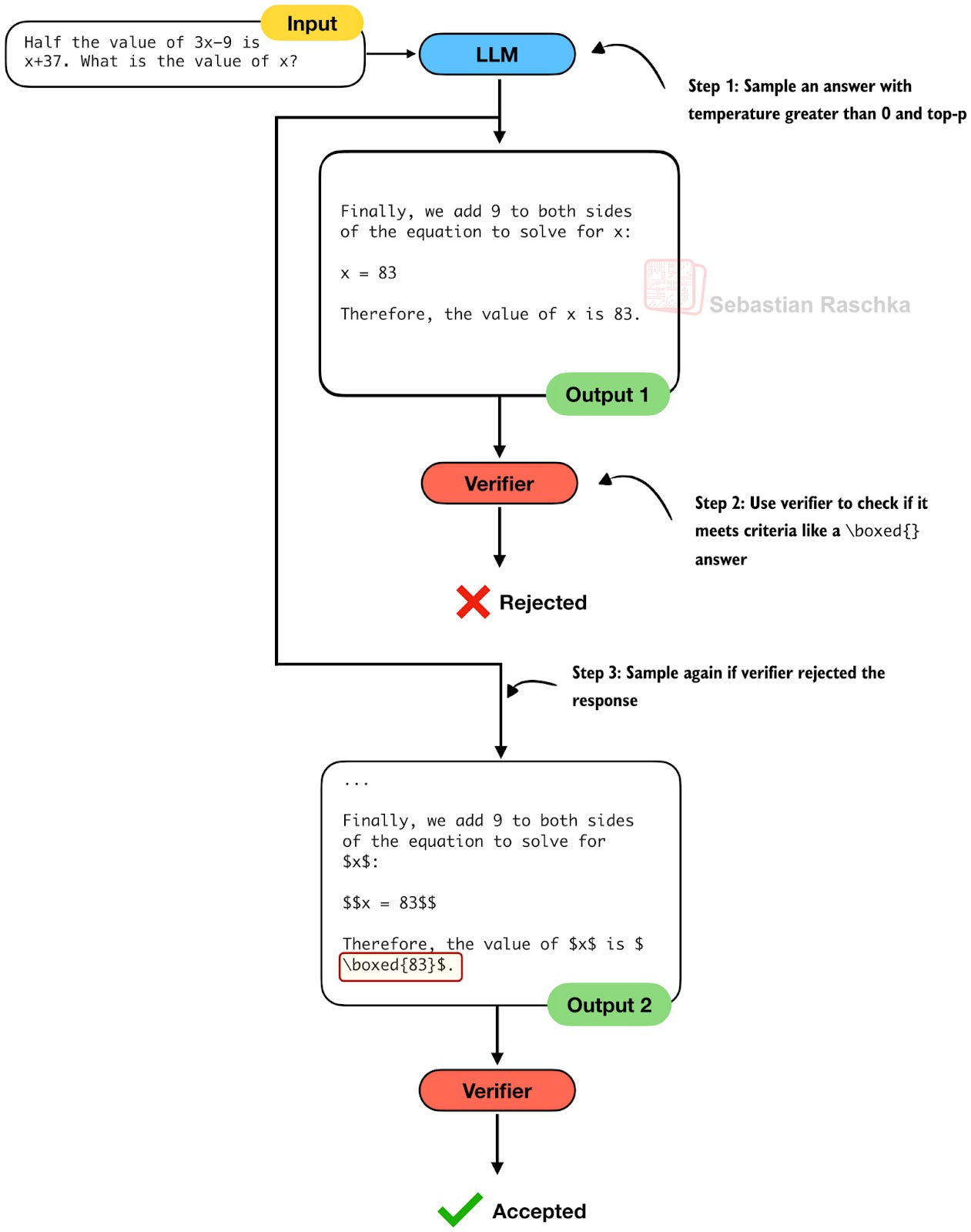
Rejection sampling is another relatively straightforward inference-scaling technique. Here, we simply repeatedly sample answers from the model until a verifier-based criterion is met. For example, think about producing a for a math problem. If a model fails to follow the instruction and doesn’t output a , we keep sampling until it either does or a maximum number of trials is met.
Figure 9: An illustration of rejection sampling.
In practice, rejection sampling serves as a helpful baseline for filtering out misformatted or otherwise instruction-violating outputs. It can also be layered on top of other inference-scaling strategies, for example as a preprocessing step before self-consistency or as a guardrail in a Best-of-N pipeline.
Rejection sampling is not only an inference-time technique. It is also embedded in many modern training pipelines. For example, DeepSeek R1 applied rule-based correctness checks, and DeepSeek V3 used its own model-as-a-judge filtering, to retain only correct or high-quality samples.
5.1 Rejection Sampling Papers (2025)
7 Apr 2025, T1: Tool-Integrated Self-Verification for Test-Time Compute Scaling in Small Language Models, https://arxiv.org/abs/2504.04718
This paper proposes a verifier-augmented Best-of-N inference scaling method. It delegates memorization-heavy checks to external tools such as a code interpreter or a retriever, and then, for the remaining ones that can’t be checked externally with tools, it self-verifies its own solutions. I.e., in short, incorrect candidates are removed before the remaining ones are scored by a reward-model verifier. (I could have added this to the Best-of-N section as well, but it already has a longer list of papers, which is why I am including it here under the rejection sampling category.)
13 Oct 2025, ROC-n-reroll: How Verifier Imperfection Affects Test-Time Scaling, https://arxiv.org/abs/2507.12399
This paper shows that the behavior of Best-of-N and rejection sampling depends entirely on the verifier’s ROC curve. In other words, given the base model’s accuracy, the ROC curve fully determines how much accuracy you gain as you increase inference-time compute.
The two main results are:
Rejection sampling is more compute-efficient than Best-of-N, though both converge to the same accuracy at very large compute.
It’s impossible to predict long-compute performance from short-compute results, because verifiers that look similar at high false positive rates often behave very differently at the low-false-positive-rate region that matters when compute increases.
- Self-Refinement
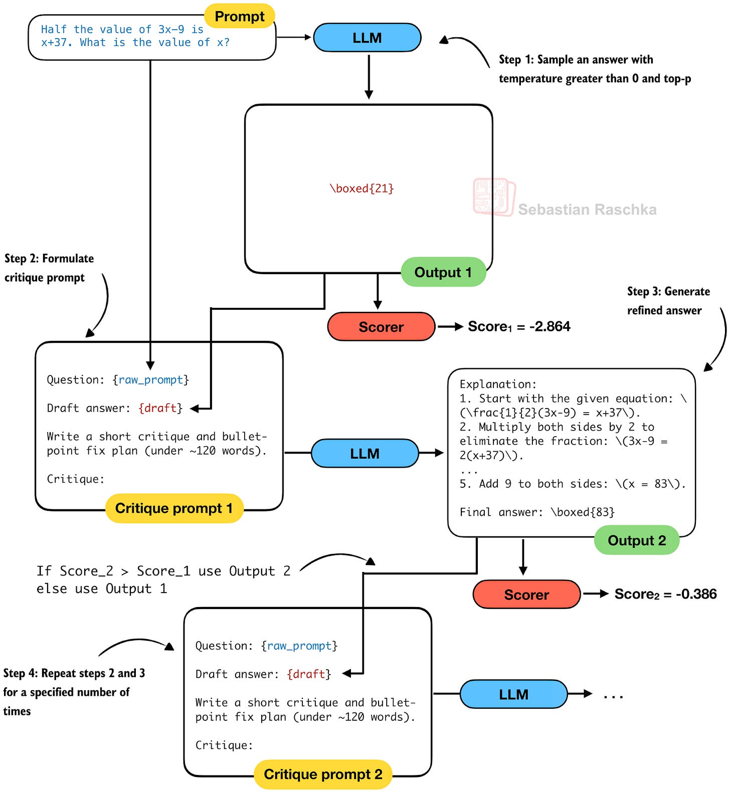
Self-refinement is an inference-time scaling strategy in which a model improves its own answers through one or more revision cycles. I’d say today this is probably the prototypical example of inference scaling in reasoning models, i.e., the first method that intuitively comes to mind when talking about improving reasoning model results.
The idea is that instead of relying on a single chain of thought, the model first produces an initial answer. Then, it generates a feedback prompt that points out potential mistakes or inconsistencies. Based on the feedback, it then regenerates a refined answer.
Figure 10: An illustration of self-refinement.
This loop (steps 2 and 3) can be repeated multiple times, with each iteration giving the model a chance to correct earlier reasoning errors, explore alternative solutions, or just improve its explanation if the answer is already correct.
Scoring-wise, as with Best-of-N, we can use a heuristic score, an LLM-as-a-judge, or log-likelihood to evaluate the answers. Using the score, we can decide at each iteration whether to accept a refinement. In a sense, this is related to rejection sampling, but the difference is that we actively refine the answer rather than just sampling again with the original prompt.
6.1 Self-Refinement Papers (2025)
8 Feb, Evolving LLMs’ Self-Refinement Capability via Synergistic Training-Inference Optimization, https://arxiv.org/abs/2502.05605
This paper asks a simple question: can an LLM reliably improve its own answers when asked to refine them? The authors first show that current models cannot. Across multiple refinement prompts, models often get worse when revising their own outputs, rather than better. (In my experience, this is only true if you do too many refinement loops.)
In this paper, the authors propose a framework to improve self-refinement capabilities with additional training. The key idea is a two-stage loop: (1) use supervised fine-tuning to activate basic self-refinement behavior, and (2) use iterative preference training to strengthen it.
22 Jan 2025, Test-Time Preference Optimization: On-the-Fly Alignment via Iterative Textual Feedback, https://arxiv.org/abs/2501.12895
This paper proposes a preference-driven form of Best-of-N. Alternatively, we can think of it as self-refinement with multiple samples, as in Best-of-N. Instead of only sampling many candidates and choosing the highest-scoring one, this method introduces an iterative refinement loop guided by a reward model. Each iteration samples several responses, scores them, compares the best and worst, and turns that comparison into textual critiques that the model then uses to rewrite its answer.
30 May, Reflect, Retry, Reward: Self-Improving LLMs via Reinforcement Learning, https://arxiv.org/abs/2505.24726
This paper proposes a preference-driven form of Best-of-N test-time scaling. Instead of only sampling many candidates and choosing the highest-scoring one, TPO introduces an iterative refinement loop guided by a reward model. Each iteration samples several responses, scores them, compares the best and worst, and turns that comparison into critiques that the model then uses to rewrite its answer.
25 Mar, Think Twice: Enhancing LLM Reasoning by Scaling Multi-round Test-time Thinking, https://arxiv.org/abs/2503.19855
This strategy iteratively improves a model’s answer by feeding back only “the final answer” from the previous round, then asking the model to “think again” and re-answer. It is essentially a more minimalistic form of self-refinement. According to the authors, only feeding the final answer, and not the reasoning trace, reduces a model’s tendency to follow the same flawed reasoning path if it sees its own chain-of-thought again.
- Search Over Solution Paths
Search over solution paths is a category name I came up with for methods in which a model explores multiple possible reasoning steps in parallel rather than committing to a single linear chain. However, unlike simple parallel sampling in self-consistency and Best-of-N, this category involves intermediate branching.
A classic example of this is beam search. Another example is Tree-of-Thoughts. The main difference between the two is in their scoring. Beam search usually uses classic log-likelihood scoring, whereas tree-of-thoughts typically uses an external scorer (like a verifier or LLM-as-a-judge). In practice, the tree-of-thought tends to work better for reasoning tasks, where the true answer is often of low likelihood.
Figure 11: An illustration of Tree-of-Thoughts sampling.
Tree-of-Thoughts generates multiple nodes at each level, and it evaluates them with a scorer to keep only expanding “the good ones” for efficiency. At the end, it evaluates the leaf nodes to select the final answer.
(Note that the figure is relatively simple in terms of branching complexity to make it fit. However, the fact that it is unbalanced is intentional. Tree-of-Thoughts does not usually produce a fixed number of branches per node. Instead, the branching factor varies depending on pruning, scoring, and budget constraints, so there may be different numbers of children at each step.)
7.1 Search Over Solution Paths Papers (2025)
6 Feb, Step Back to Leap Forward: Self-Backtracking for Boosting Reasoning of Language Models, https://arxiv.org/abs/2502.04404
This paper operates on the same underlying idea as Tree-of-Thoughts, namely, reasoning as a search process over a tree of intermediate steps.
In Tree-of-Thoughts, the model proposes multiple partial reasoning steps; these steps form nodes in a search tree, and an external scorer decides when to branch or prune (or backtrack). The self-backtracking paper uses exactly this structure.
But where Tree-of-Thoughts performs search externally using a scorer, the self-backtracking method instead trains the model to internalize part of the search algorithm. So, the model learns to recognize when a reasoning path is invalid and explicitly emits a
This makes it essentially a learned form of Tree-of-Thought-style search.
16 Oct 2025, Reasoning with Sampling: Your Base Model Is Smarter Than You Think, https://arxiv.org/abs/2510.14901
The authors introduce an iterative sampling approach based on Markov Chain Monte Carlo (MCMC) to obtain better reasoning traces from a base model without any external scorers or verifiers. It’s somewhat similar to beam search or Tree-of-Thoughts, since both aim to move the generated text toward higher-likelihood trajectories via branching decisions.
The key difference is that beam search and Tree-of-Thoughts explicitly keep several branches in parallel. In contrast, this MCMC-based method never explicitly maintains multiple trajectories. Instead, it works with a single sequence and repeatedly resamples subsequences. So, at branching points (blocks of tokens) it accepts or rejects each proposal based on its likelihood under the base model. So, in the end, we have a single-path, stochastic search procedure that creates a single reasoning path.
Ultimately, it’s a flavor of Tree-of-Thoughts with MCMC sampling.
7 Feb, Adaptive Graph of Thoughts: Test-Time Adaptive Reasoning Unifying Chain,
Tree, and Graph Structures, https://arxiv.org/abs/2502.05078
This Graph-of-Thoughts paper can be seen as a generalization of Tree-of-Thoughts, creating a directed acyclic graph instead of a tree.
And where Tree-of-Thoughts relies on an external scorer or verifier to decide which branches to expand, the Graph-of-Thoughts approach lets the model itself determine when a thought is “complex” and should trigger a nested subgraph.
7 Aug 2025, DOTS: Learning to Reason Dynamically in LLMs via Optimal Reasoning Trajectories Search, https://arxiv.org/abs/2410.03864
This paper shares the same high-level perspective as Tree-of-Thoughts, namely that different questions benefit from different reasoning trajectories rather than a single fixed pattern. But instead of branching over partial solutions (as in Tree-of-Thoughts), DOTS branches over reasoning actions such as rewriting, chain-of-thought, self-verification, and others.
The method systematically searches these action sequences to find an optimal trajectory for each prompt. However, before this, the model performs this search during inference, which requires training the model for this behavior.
31 Dec 2025, Recursive Language Models, https://arxiv.org/abs/2512.24601
This is one of the most promising papers I’ve seen, and I think we will see more of that in 2026.
This paper reframes long-context inference as an “out-of-core” problem. Instead of feeding an enormous prompt into the LLM, the prompt is treated as an external object that can be programmatically inspected and sliced.
Concretely, in a Python REPL environment, the model writes code to analyze and chunk the prompt, recursively invokes sub-LLM calls on shorter prompt snippets, and then stitches the intermediate results back together.
9 Jan 2026, PaCoRe: Learning to Scale Test-Time Compute with Parallel Coordinated Reasoning, https://arxiv.org/abs/2601.05593
This paper treats reasoning as a search over solution paths, in the same spirit as Tree-of-Thoughts.
However, instead of growing a single search tree inside the context window, PaCoRe scales search through parallel exploration. More concretely, this means that the model generates many reasoning trajectories in parallel, then compresses their conclusions into short messages, and then uses those messages to guide the next round of exploration.
7.2 A Closer Look at Recursive Language Models (RLMs)
Since the Recursive Language Models (RLM) paper (https://arxiv.org/abs/2512.24601), which is listed above, made such big waves a few weeks ago, I wanted to expand a bit on that and explains what it is and how it works.
7.2.1 Handling Long Contexts by Chunking Prompts for LLM Subcalls
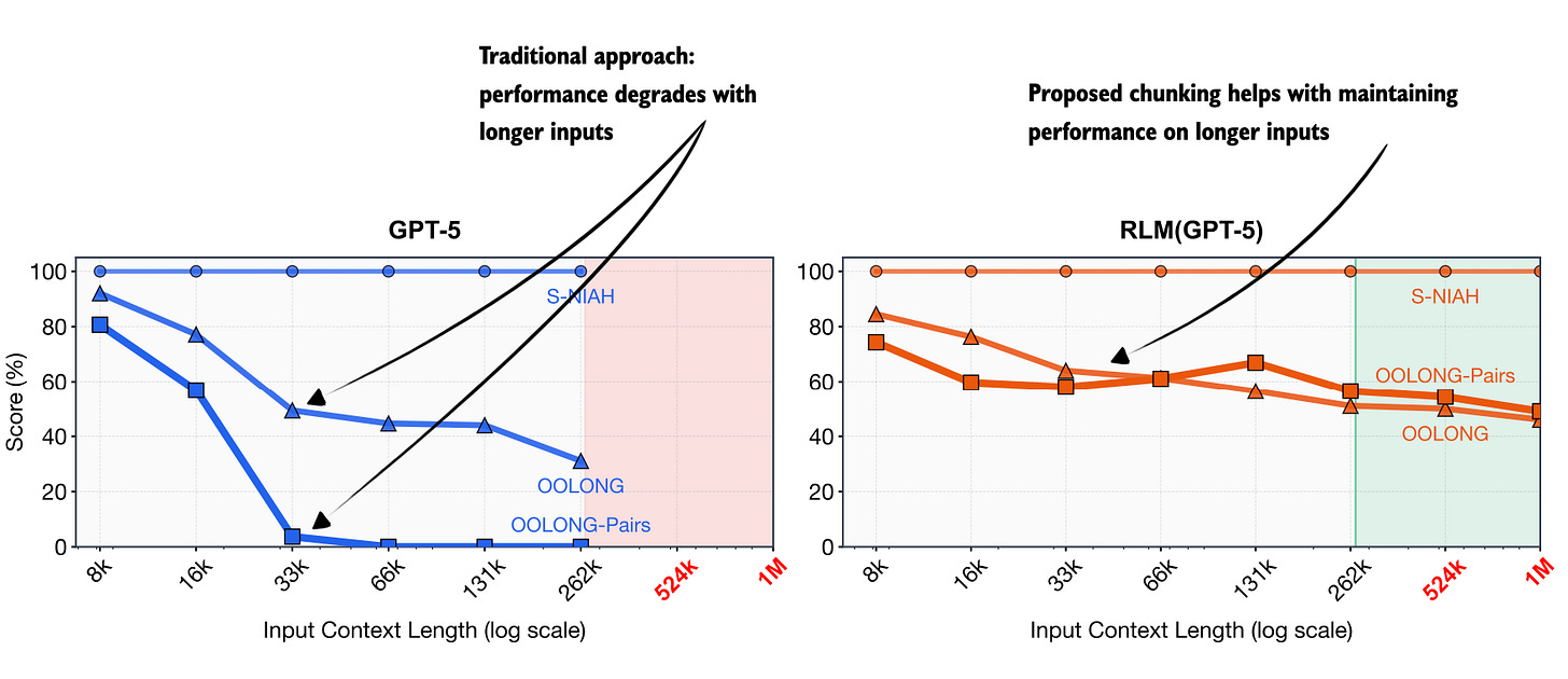
The key motivation is the observation that LLMs perform worse as input length increases. This is partly related to the known, classic “needle-in-the-haystack” problem, as an increasing number of token inputs can bury the important information and/or distract the LLM.
However, the motivation for this approach goes also beyond classic needle-in-a-haystack failures. For instance, the authors argue that performance degradation in long-context settings depends not only on input length, but also on task complexity. And tasks that require repeated, targeted access to distant parts of the input tend to suffer most from context rot.
Annotated figure from the RLM paper, https://arxiv.org/abs/2512.24601
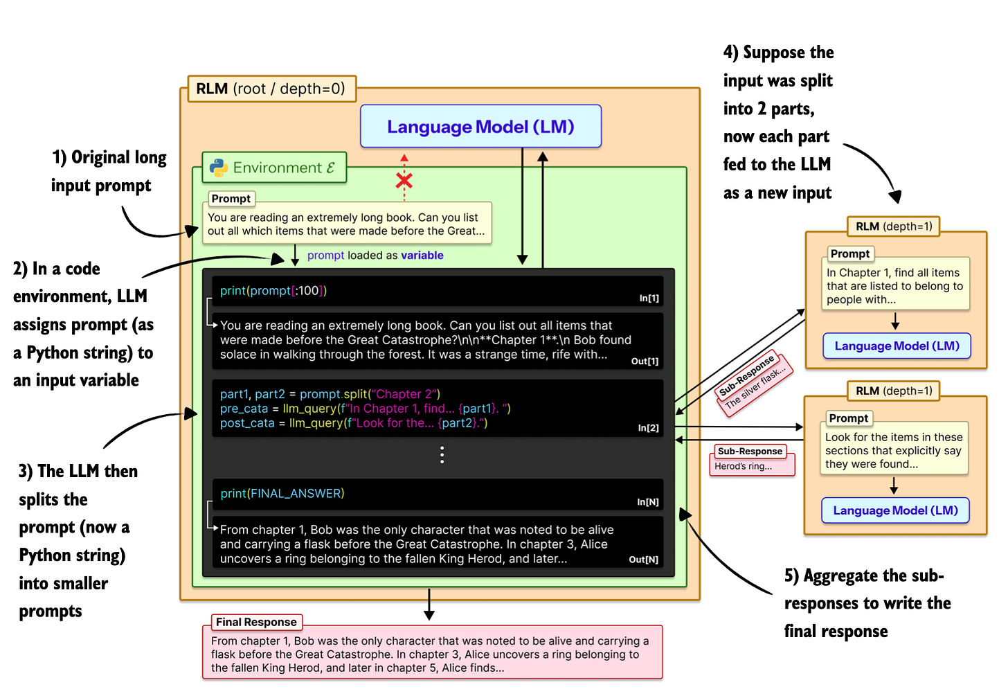
So, to improve the performance on longer contexts, the authors of the RLM paper propose an inference-time alternative to extending context windows. Instead of feeding a very long prompt directly into the model, the full input is placed into an external execution environment (like a Python REPL). The LLM then writes code to inspect, filter, chunk, and selectively process this input, recursively (by invoking more LLM calls using smaller, filtered and chunked inputs).
Annotated figure from the RLM paper, https://arxiv.org/abs/2512.24601
As more or less illustrated in the figure above, a key point is that RLMs are not merely about chunking long prompts and running the model on each chunk. While simple chunking is one possible strategy, the core idea is to let the model interact programmatically with the input.
Or, in other words, the novelty lies in treating the long input as out-of-core data that the model can manipulate programmatically to best do these recursive subcalls.
This approach can be seen as inference-time compute scaling with variable cost. In the paper’s setup, a stronger “root” model orchestrates the process, while cheaper sub-models handle recursive calls. This keeps median costs comparable to standard prompting, but it can also increase the costs depending on depth of the recursive calls and cost of the sub-models.
7.2.2 Does This RLM Approach Work for Reasoning Tasks?
In my view, the RLM technique is a great approach for knowledge-heavy tasks that involve a lot of Q&A-like tasks (like anything that involves looking up and verifying information).
However, I suspect this RLM approach would not work well for typical reasoning tasks like math (e.g., MATH-500 style math questions) that need to be solved sequentially, where each step depends on the previous one. (But to be fair, the focus and advantage of this RLM method is not long outputs but rather long, information-dense inputs.)
On the other hand, on coding tasks, I can see this method excel, especially when working with larger code bases that involve multiple files. Here, it would make absolute sense to have the LLM process things in parallel via recursive subcalls rather than sequentially. But again, for short snippets or functions, it has the same limitation as mentioned for the math tasks above.
All in all, it’s an exciting method to start this year with.
- Conclusions, Categories, and Combinations
I wanted to define and focus on a few core categories. Even though not all papers (and other flavors of these methods) fall neatly under these categories, I think this is a more or less helpful way to think about inference-scaling. I.e., as mentioned earlier, at its core, inference scaling is about expending more compute and/or time (or, simply, more tokens) to improve the model’s responses.
The categories covered in this article were:
Chain-of-thought prompting, which simply asks the model to generate explanations
Self-consistency, which is about trying it / generating answers multiple times
Best-of-N, which can be thought of as an extension of self-consistency, but we actively score the answers to select the best one
Rejection sampling, which is about throwing out bad answers that violate guidelines or instructions, or have any other automatically detectable issues
Self-refinement, which is an iterative technique that sequentially improves the answer
Search over solution paths, which is an umbrella technique that explores different answers by branching out
8.1 Parallel and Sequential Techniques
We can further categorize the techniques into parallel and sequential sampling techniques. Here, “parallel” means we can generate all answers simultaneously. So, if we have the necessary compute resources, we don’t incur latency penalties, which can be important in certain applications.
Self-consistency and Best-of-N are clearly parallel strategies.
Rejection sampling can be parallel, but it would produce many wasteful generations if we don’t combine it with Best-of-N-style scoring.
On the other hand, chain-of-thought prompting is clearly a sequential method. Sequential means we generate more tokens iteratively. If it makes the model generate 4x more tokens, it will be 4x slower.
Self-refinement, while being a powerful technique that bootstraps the model to (more or less) improve itself, is also an inherently sequential method.
Lastly, search over solutions paths is an interesting mix between parallel and sequential, where we switch between growing the trajectory (sequential) and parallel (branching and growing each trajectory independently).
8.2 Combinations
Of course, we can also combine most of these methods, meaning we can use more than one at a time. Most combinations are intuitive and further improve performance. However, the more we combine these methods, the more expensive inference scaling gets.
To provide one of the many example scenarios, we could use self-consistency as our baseline for solving math problems. For each independent sample in self-consistency, we could use self-refinement over several iterations and then extract the final answer. Additionally, we can use a Best-of-N-style scoring method if there are ties in self-consistency sampling (for instance, if our possible answers are [4, 4, 2, 3, 2]).
8.3 The Best Method?
The big question in the room, though, is which techniques to use? I have tried all the main categories covered in this article. In addition, I also tried some of the research techniques mentioned here.
For each method, I tried a few hyperparameter settings, like changing the sample size in self-consistency or the number of iterations in self-refinement. I also tried different scoring methods from heuristics (based on whether the boxed answer can be extracted, how long the answer is, etc.) to log-likelihood scoring and LLM-as-a-judge.
Then, I also combined several methods, like Best-of-N with self-refinement, etc.
However, I must admit that, due to budget constraints, I didn’t exhaustively test all combinations and reasonable hyperparameter configurations. I also only evaluated these methods on MATH-500 and used a small Qwen 0.6B Base model. Even then, this amounted to approximately a thousand runs.
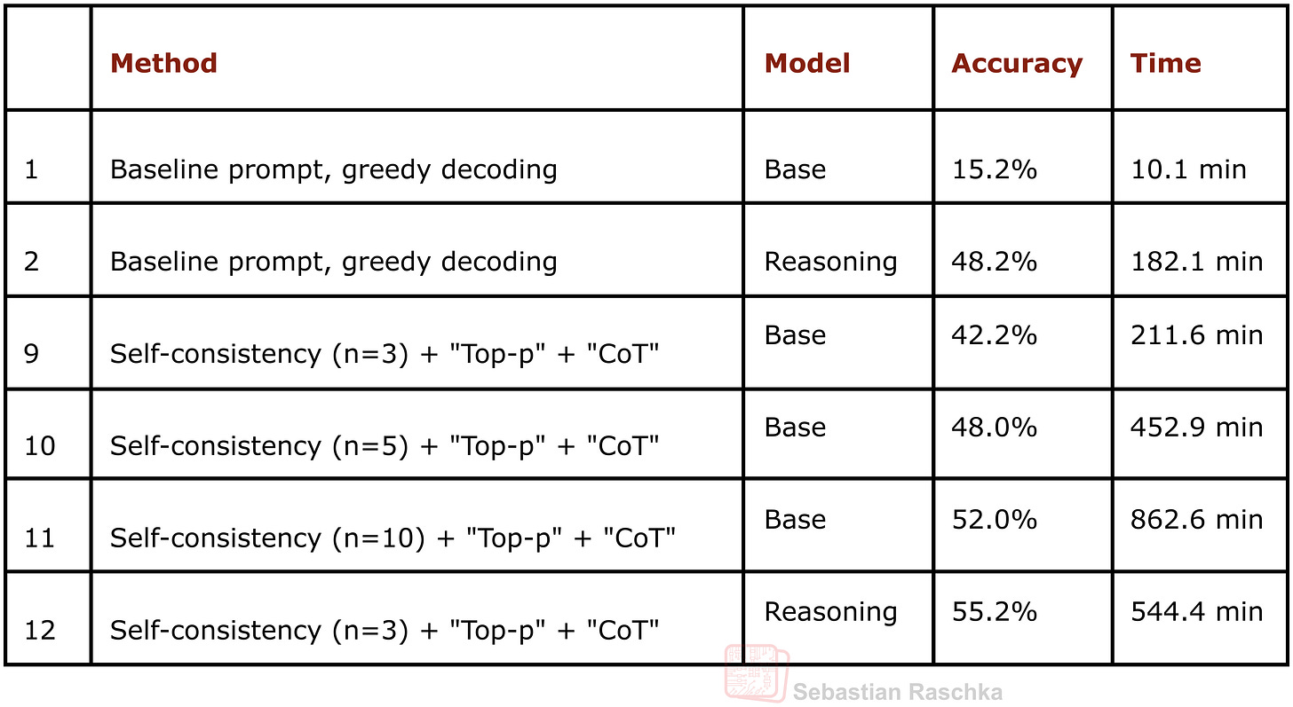
That said, given these limitations, I found that self-consistency was the best method. However, “best” is a big word since even in the self-consistency category, changing the sample size has a big impact on both accuracy and runtime. For example, yes, you can boost the base model’s accuracy from 15.2% to 52.0% by combining self-consistency with chain-of-thought prompting and using a sample size of 10. But is the 4x increased runtime over self-consistency with a sample size of 3 and accuracy of 42.2% worth it?
Figure 12: An excerpt of an earlier table showing the performance of the baselines without inference scaling (rows 1 and 2) and several flavors of self-consistency (rows 9-12).
In addition to the code for the experiments above, I may share the code and results of other methods over time in my GitHub repo at https://github.com/rasbt/reasoning-from-scratch.
If you are planning to experiment with inference scaling, my recommendation is to start with self-consistency as a baseline, try self-refinement, and tune different knobs. Then consider adding other methods one by one and see if they improve. Here, improvements mean the same accuracy, lower resource use or runtime, or, at a fixed runtime, higher accuracy.
All that being said, take this with a grain of salt, as it may look very different across model sizes, model types, and benchmark datasets.
- Bonus: What Do Proprietary LLMs Use?
We can all agree that the main deployed LLMs use some sort of inference scaling. E.g., as discussed at the beginning of this article, the accuracy improvements due to inference scaling were specifically highlighted in the o1 reasoning model release in OpenAI’s blog post.
Unfortunately, it’s hard to say what exactly OpenAI, Anthropic, Google, xAI, etc., use in their platforms. However, based on publicly available information, it may be worth speculating a bit.
9.1 Chain-of-Thought
To quote from the OpenAI o1 system card:
“One of the key distinguishing features of o1 models are their use of chain‑of‑thought when attempting to solve a problem”
So, yes, OpenAI’s o1 model (as well as the GPT-5 and GPT-5.1) models use some form of internal chain-of-thought. Note that these models have been specifically trained to emit these chains (similar to DeepSeek R1, for example), so we don’t have to use prompt tricks like “Explain step by step.”
In other words, the “thinking” is already built in (and there are additional options, via the system prompt, to regulate how much “thinking” should be used; their gpt-oss open-weight model supports this sort of “thinking budget” as well.)
Also, Gemini Pro 3, Grok 4.1, and Claude Opus 4 all have similar reasoning models that emit chains-of-thought.
9.2 Self-Consistency and Best-of-N
It’s hard to say if OpenAI uses these techniques for regular prompts. However, at least they use them for their benchmarks. According to the o1 blog:
o1 averaged 74% (11.1/15) with a single sample per problem, 83% (12.5/15) with consensus among 64 samples, and 93% (13.9/15) when re-ranking 1000 samples with a learned scoring function.
Anthropic seems to be even more explicit about the use of self-consistency and Best-of-N in their evaluations:
Our researchers have also been experimenting with improving the model’s performance using parallel test-time compute. They do this by sampling multiple independent thought processes and selecting the best one without knowing the true answer ahead of time. One way to do this is with majority or consensus voting; selecting the answer that appears most commonly as the ‘best’ one. Another is using another language model (like a second copy of Claude) asked to check its work or a learned scoring function and pick what it thinks is best (Source)
Next, from the Grok 4 blog article:
We have made further progress on parallel test-time compute, which allows Grok to consider multiple hypotheses at once. We call this model Grok 4 Heavy, and it sets a new standard for performance and reliability.
Gemini also announced in December a mode that sounds just like self-consistency or Best-of-N:
We’re pushing the boundaries of intelligence even further with Gemini 3 Deep Think. This mode meaningfully improves reasoning capabilities by exploring many hypotheses simultaneously to solve problems.
9.3 Rejection Sampling
I could not find any public information on the use of rejection sampling in the aforementioned proprietary, deployed LLMs. However, rejection sampling being a useful “add-on” technique, I suspect that this is simply too trivial to talk about.
I think where it finds the most use is in a) the training pipeline (as part of the reinforcement learning with verifiable rewards part) and b) for safety filtering, where certain LLM answers or answer segments may get flagged.
9.4 Self-Refinement and Search Over Solution Paths
I am fairly confident that self-refinement and search over solution paths are popular techniques in proprietary reasoning models.
Again, to quote from the OpenAI o1 Learning to Reason blog post:
“learns to recognize and correct its mistakes” and “learns to try a different approach when the current one isn’t working.”
The above sounds like a clear example of a combination of self-refinement and search over solution paths.
Unfortunately, I could not find any additional information about the other proprietary LLMs. However, self-refinement is, I think, a no-brainer when reading through the reasoning traces output by the LLM.
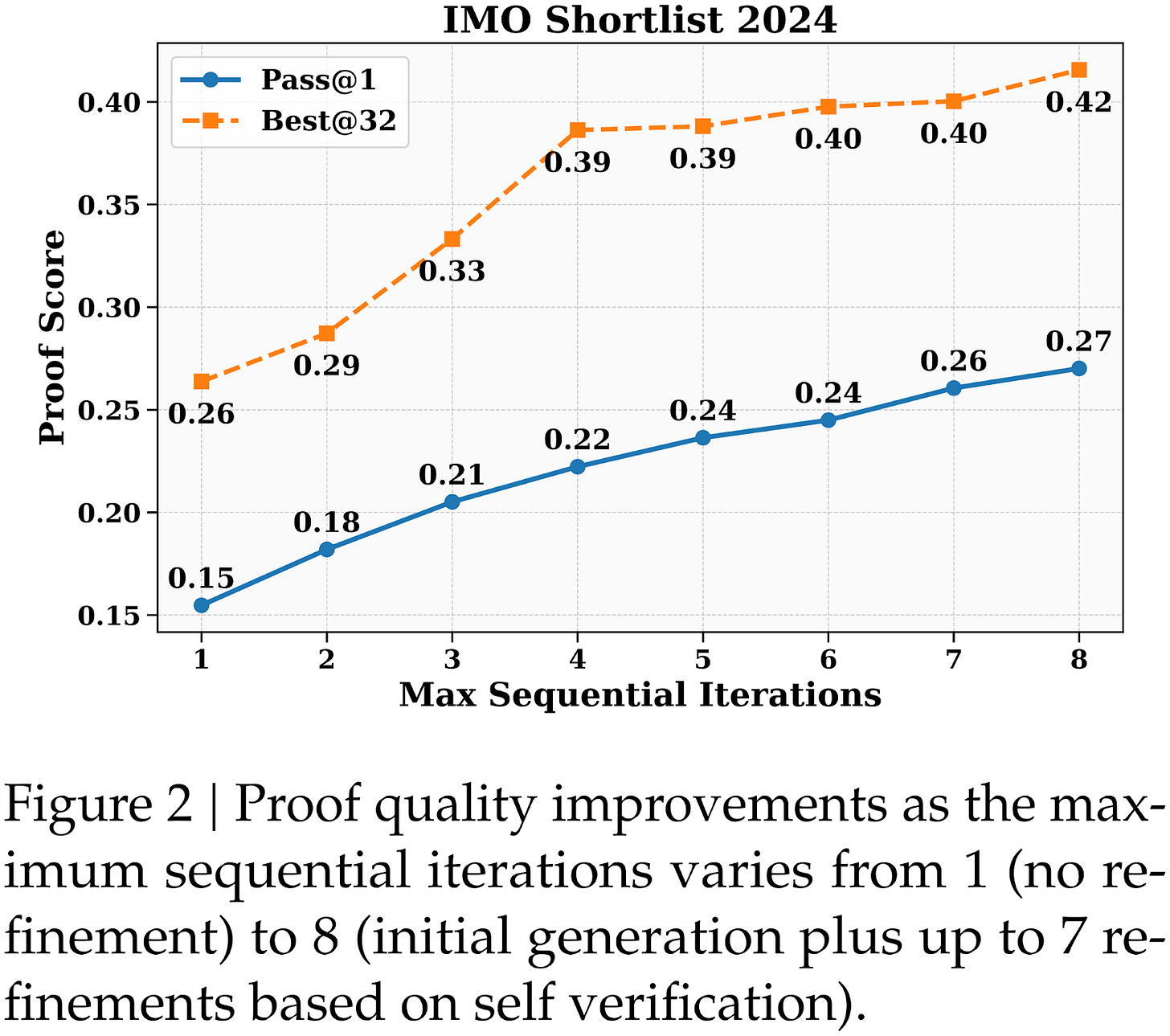
Related to this, DeepSeek also just released a new model, DeepSeekMath-V2, which is more explicitly using self-refinement as an external loop, similar to what we discussed in section 5:
Our model can assess and iteratively improve its own proofs
This allows a proof generator to iteratively refine its proofs until it can no longer identify or resolve any issues.
Figure 13: Figure from the DeepSeekMath-V2 report showing how the answer improves with an increasing number of self-refinement iterations.
Even when details are sparse, the behavior we see in model traces strongly suggests that self-refinement and search over solutions paths are now standard practice. My sense is that these techniques will continue to play an essential role as we push reasoning models toward greater robustness and reliability.
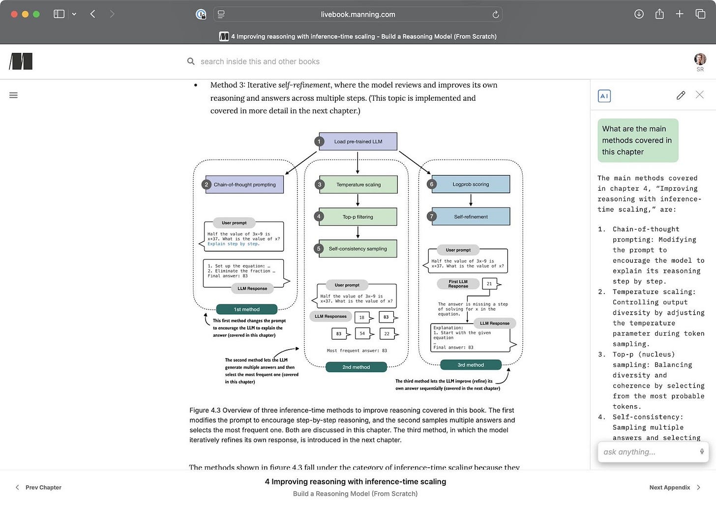
It’s been a long article, and I hope you found this overview of inference scaling useful. If you want a more detailed coverage with step-by-step, from-scratch code, chapters 4 of Build a Reasoning Model (From Scratch) implements self-consistency along with temperature scaling and top-p sampling. Chapter 5 then builds on this foundation with log-probability scoring and self-refinement.
Excerpt of chapter 4 in Build a Reasoning Model (From Scratch)
Thanks for reading, and thanks for the kind support! – Sebastian Raschka