Understanding and Implementing Qwen3 From Scratch

Subtitle: A Detailed Look at One of the Leading Open-Source LLMs

Date: JUL 19, 2025

URL: https://magazine.sebastianraschka.com/p/qwen3-from-scratch

Likes: LIKE (4)

Image Count: 21

---

Images

1. 

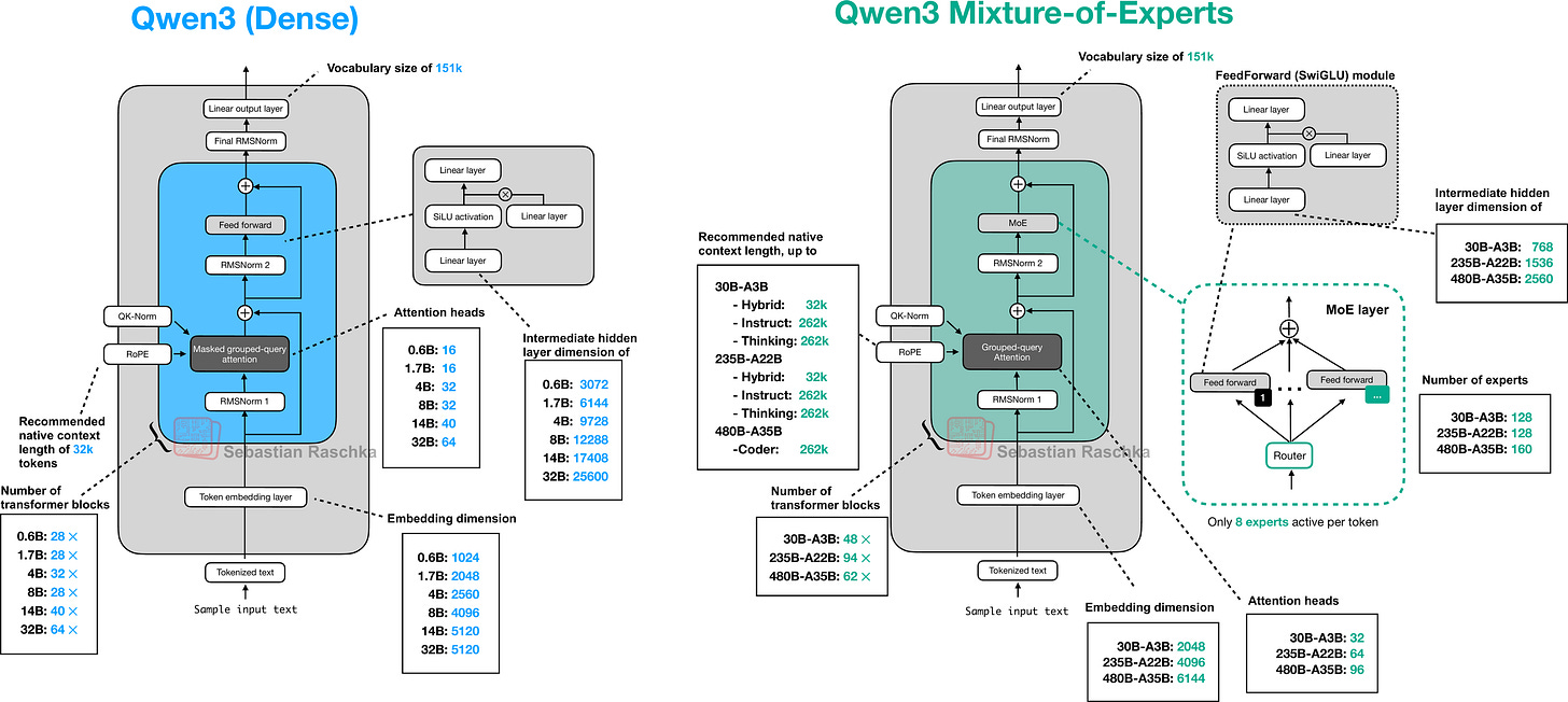
   Figure

   • Caption: Figure 1: Preview of the Qwen3 Dense and Mixture-of-Experts architectures discussed and (re)implemented in pure PyTorch in this article.

2. 

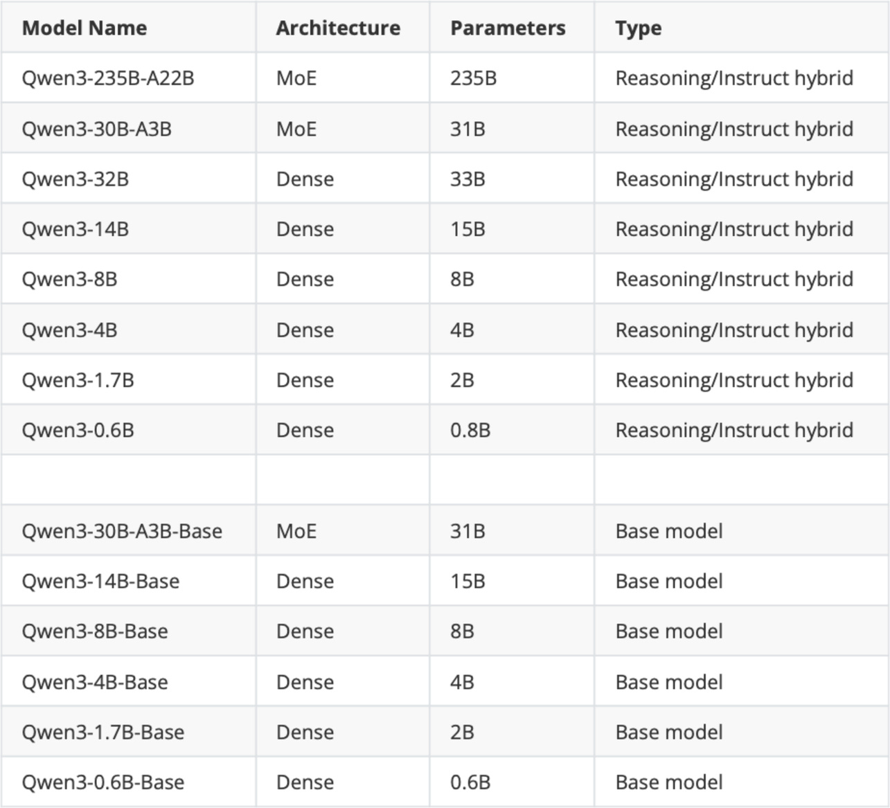
   Figure

   • Caption: Figure 2: The original Qwen3 model suite released in May 2025.

3. 

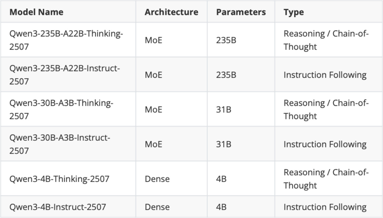
   Figure

   • Caption: Figure 3: The updated Qwen3 models that were released on July 25.

4. 

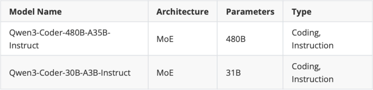
   Figure

   • Caption: Figure 4: Qwen3 code models.

5. 

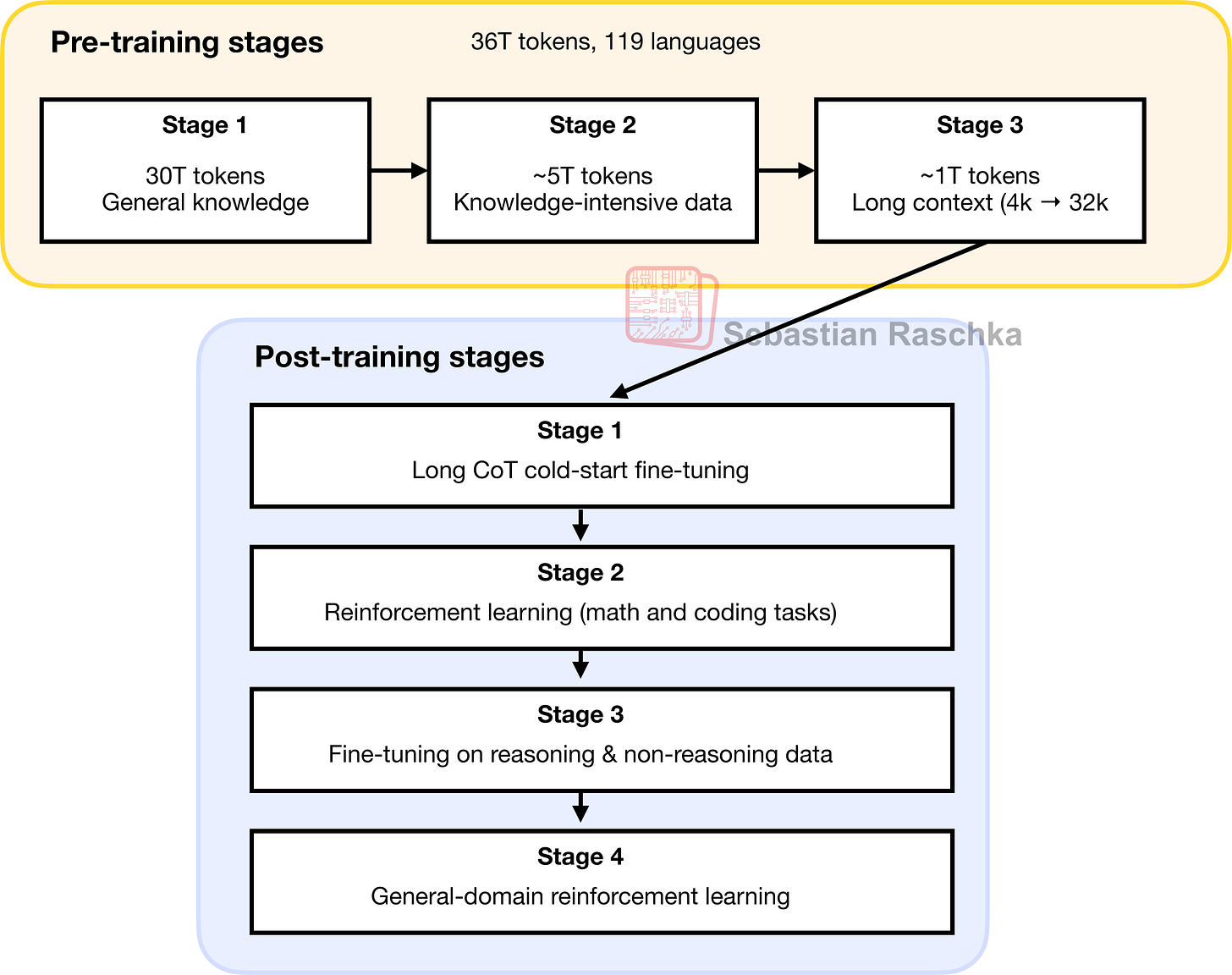
   Figure

   • Caption: Figure 5: A visual summary of Qwen3’s pre- and post-training stages.

6. 

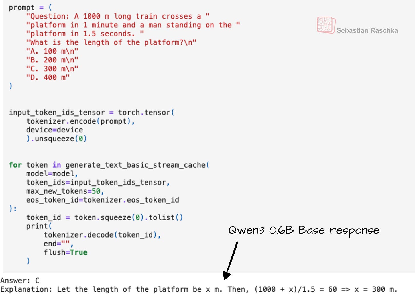
   Figure

   • Caption: Figure 6: Even when given a simple multiple-choice question (here from MMLU), the Qwen3 0.6B base model provides an explanation along with the answer, which is atypical for base models and likely a consequence of including chain-of-thought data in the pre-training mix.

7. 

   Figure

   • Caption: Figure 7: The Qwen3 post-training stages mapped onto the DeepSeek R1 training pipeline.

8. 

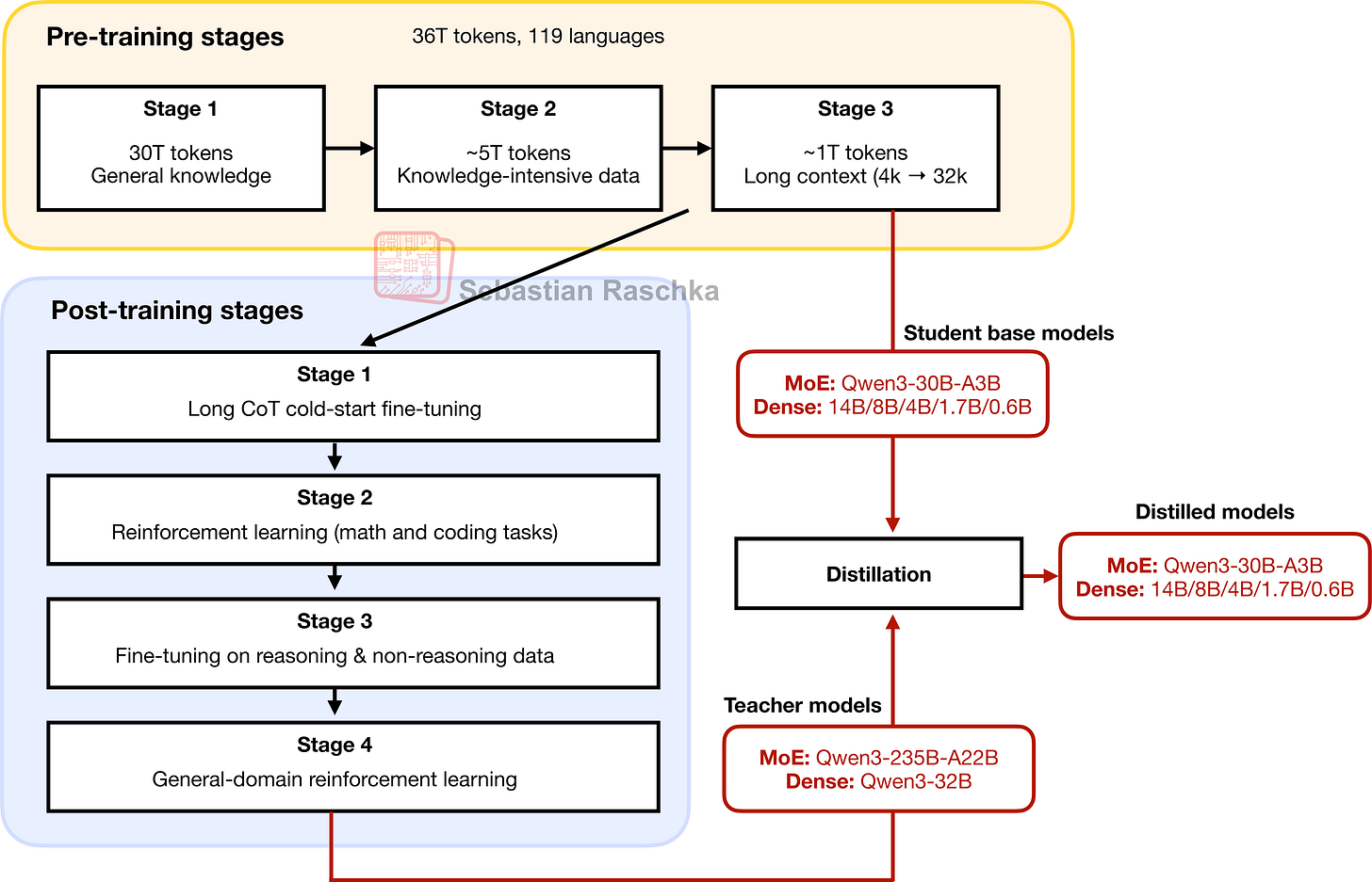
   Figure

   • Caption: Figure 8: The smaller Qwen3 MoE and dense models are distilled from the largest MoE and largest dense model, respectively.

9. 

   Figure

   • Caption: The Big LLM Architecture Comparison

10. 

    Figure

• Caption: Figure 9: Architectural comparison between Qwen3 0.6B and the 127M parameter GPT-2 variant. Both models process text through embedding layers and stacked transformer blocks, but they differ in certain design choices.

11. 

    Figure

• Caption: Figure 10: Comparison of LayerNorm and RMSNorm. LayerNorm (left) normalizes activations so that their average value (mean) is exactly zero and their spread (variance) is exactly one. RMSNorm (right) instead scales activations based on their root mean square, which does not enforce zero mean or unit variance, but still keeps the mean and variance within a reasonable range for stable training.

12. 

    Figure

• Caption: Figure 11: In GPT-2 (top), the feed forward module consists of two fully connected (linear) layers separated by a non-linear activation function. In Qwen3 (bottom), this module is replaced with a gated linear unit (GLU) variant, which adds a third linear layer and multiplies its output elementwise with the activated output of the second linear layer.

13. 

    Figure

• Caption: Figure 12: Different activation functions that can be used in a feed forward module (neural network). GELU and SiLU (Swish) offer smooth alternatives to ReLU, which has a sharp kink at input zero.

14. 

    Figure

• Caption: Figure 13: Illustration of the RoPE two-halves variant. Here, it shows how a position pair in the query (or key) vector is rotated via a rotation angle α_{i,j}, which is based on a position i and a frequency constant ω_j. The figure is inspired by Figure 1 in the original RoPE paper.

15. 

    Figure

• Caption: Figure 14: A comparison between MHA and GQA. Here, the group size is 2, where a key and value pair is shared among 2 queries.

16. 

    Figure

• Caption: Figure 15: The Structure of the transformer block in Qwen3. Each block includes RMSNorm, RoPE, masked grouped-query attention, and a feed-forward module, and is repeated 28 times in the 0.6B-parameter model.

17. 

    Figure

• Caption: Figure 16: Architecture of the Qwen3 0.6B model. The model consists of a token embedding layer followed by 28 transformer blocks, each containing RMSNorm, RoPE, QKNorm, masked grouped-query attention with 16 heads, and a feed-forward module with an intermediate size of 3,072.

18. 

    Figure

• Caption: Figure 17: Speed-comparison between a regular and KV cache implementation of Qwen3 0.6B.

19. 

    Figure

• Caption: Figure 18: The typical one-token-at-a-time text-generation pipeline of an LLM with KV cache.

20. 

    Figure

• Caption: Figure 20: The Qwen3 MoE architecture.

21. 

    Figure

• Caption: Figure 21: Visual overview of the Build a Reasoning Model (From Scratch) book.

---

Full Text Content

Previously, I compared the most notable open-weight architectures of 2025 in The Big LLM Architecture Comparison. Then, I zoomed in and discussed the various architecture components in From GPT-2 to gpt-oss: Analyzing the Architectural Advances on a conceptual level.

Since all good things come in threes, before covering some of the noteworthy research highlights of this summer, I wanted to now dive into these architectures hands-on, in code. By following along, you will understand how it actually works under the hood and gain building blocks you can adapt for your own experiments or projects.

For this, I picked Qwen3 (initially released in May and updated in July) because it is one of the most widely liked and used open-weight model families as of this writing.

The reasons why Qwen3 models are so popular are, in my view, as follows:

A developer- and commercially friendly open-source (Apache License v2.0) without any strings attached beyond the original open-source license terms (some other open-weight LLMs impose additional usage limits)

The performance is really good; for example, as of this writing, the open-weight 235B-Instruct variant is ranked 8 on the LMArena leaderboard, tied with the proprietary Claude Opus 4. The only 2 other open-weight LLMs that rank higher are DeepSeek 3.1 (3x larger) and Kimi K2 (4x larger). On September 5th, Qwen3 released a 1T parameter “max” variant on their platform that beats Kimi K2, DeepSeek 3.1, and Claude Opus 4 on all major benchmarks; however, this model is closed-source for now.

There are many different model sizes available for different compute budgets and use-cases, from 0.6B dense models to 480B parameter Mixture-of-Experts models.

This is going to be a long article due to the from-scratch code in pure PyTorch. While the code sections may look verbose, I hope that they help explain the building blocks better than conceptual figures alone!

Tip 1: If you are reading this article in your email inbox, the narrow line width may cause code snippets to wrap awkwardly. For a better experience, I recommend opening it in your web browser.

Tip 2: You can use the table of contents on the left side of the website for easier navigation between sections.

Figure 1: Preview of the Qwen3 Dense and Mixture-of-Experts architectures discussed and (re)implemented in pure PyTorch in this article.

1 Qwen3 Model Family Overview

Before we go over the step-by-step Qwen3 implementation, a quick note: “Qwen3” is a family, not a single model. It comes in multiple sizes and in both dense and MoE variants. The initial release in May included the models listed in the table below, with additional updates in July.

Figure 2: The original Qwen3 model suite released in May 2025.

In Figure 2, 

“MoE” is short for Mixture-of-Experts, and “Dense” is the regular, non-MoE models;

“Base” means pre-trained (but not fine-tuned) base model;

“Reasoning/Instruct hybrid” means that the model can be either used as a Chain-of-Thought (CoT)-style reasoning model or a regular instruction-following model; a user can choose the behavior by adding tags, as we will see later.

Then, later in July, a week after the Kimi K2 release, the Qwen3 team updated some of its models, as shown in Figure 3:

Figure 3: The updated Qwen3 models that were released on July 25.

(On September 5th, Qwen3 released a 1T parameter “max” instruct variant on their platform that beats Kimi K2, DeepSeek 3.1, and Claude Opus 4 on all major benchmarks. However, this model is closed-source for now, so it’s not further discussed in this article as there is no public information available about it yet. However, I suspect that it is simply a scaled up version of the 235B-A22B model, that is, an MoE with 96B active parameters.)

As Figure 3 shows, Qwen3 now ships separate instruction-following (“instruct”) and reasoning (“thinking”) models rather than hybrids. The “2507” in the model name stands for the July 25 release.

A quick timeline for context:

Pre-Qwen3: Qwen2.5 offered distinct instruction-following and reasoning (QwQ) models.

May: the first Qwen3 suite introduced a hybrid reasoning model.

July 25: the team split Qwen3 into separate instruct and reasoning variants.

The shift away from hybrids is notable because DeepSeek moved in the opposite direction. It began with separate models (V3 base and R1 reasoning) and later introduced a hybrid with toggled thinking modes (V3.1).

In my experience, specialization tends to win. Training a base for instruction following and then further for reasoning usually improves reasoning, but can slightly diminish pre-training knowledge and some instruction behavior. So, separate lines avoid that compromise.

On the other hand, hybrids are attractive in production since a single served model can toggle reasoning on or off. (We don’t have to load two separate sets of model weights into memory.)

In short, separate models may result in slightly better task (or at least benchmark) performance, while hybrids simplify serving.

Lastly, the Qwen3 team also released two instruction-following models specialized for coding tasks:

Figure 4: Qwen3 code models.

All Qwen3 models can handle code to some extent, but the Qwen3-Coder models (listed in Figure 4) are additionally fine-tuned on coding tasks. This gives them more specialized behavior on coding tasks compared to the general-purpose models.

I think this is a smart design choice. If you are building or integrating code into a specific application, it usually makes more sense to use a specialized model than a general-purpose “jack-of-all-trades” model, which inevitably involves compromises.

This observation ties back to a research paper I discussed last year, which showed that fine-tuning or further pre-training an LLM on one domain tends to degrade its performance in another. For example, training on math problems improves reasoning in that area but reduces coding performance, and the reverse is true when the model is tuned for coding.

2 Training Methodology

Lastly, before we finally get to the from-scratch implementation of Qwen3, I want to summarize the training pipeline that was used to develop the models discussed in the previous section.

According to the Qwen3 technical report, the pre- and post-training consists of several stages each, which I summarized in Figure 5 below.

Figure 5: A visual summary of Qwen3’s pre- and post-training stages.

Note that the steps shown in Figure 5 correspond to the Qwen3 base and hybrid models released in May. There was no separate paper for the separate reasoning and instruct variants released in July. However, I suspect the reasoning model includes all these steps except post-training stage 3. And the Instruct model includes all these steps except for post-training stages 1 and 2.

Overall, the pre-training stages depicted in Figure 5 look fairly standard. The interesting aspect here is that in Stage 2, the Qwen3 team explicitly included knowledge-intensive (chain-of-thought-style) data, which is said to enhance reasoning capabilities later on. Nowadays, I suspect that most pre-training datasets already contain such data incidentally (as it is present in internet corpora), but the explicit inclusion is still interesting.

Personally, I have observed that the Qwen3 base models (before being post-trained for reasoning) already exhibit some reasoning behavior, as shown in Figure 6. This is likely a consequence of the pre-training data mix.

Figure 6: Even when given a simple multiple-choice question (here from MMLU), the Qwen3 0.6B base model provides an explanation along with the answer, which is atypical for base models and likely a consequence of including chain-of-thought data in the pre-training mix.

Now, coming back to the post-training pipeline shown in Figure 5, this post-training looks pretty straightforward: 

Stage 1: Supervised fine-tuning on chain-of-thought data

Stage 2: Reinforcement learning with verifiable rewards

Stage 3: more supervised fine-tuning (this time including general, non-reasoning data to support the reasoning/instruct hybrid behavior)

Stage 4: General-domain reinforcement learning

These 4 stages are essentially similar to DeepSeek R1. I tried to overlay the Qwen3 stages onto the DeepSeek R1 approach in Figure 7 below.

Figure 7: The Qwen3 post-training stages mapped onto the DeepSeek R1 training pipeline.

Note that the DeepSeek R1 pipeline looks more complex than Qwen3’s, mainly because the data generation steps are explicitly shown for DeepSeek. 

The biggest difference is at Stage 4: Qwen3’s report describes this as general-domain reinforcement learning, but it is unclear whether verifiable rewards were used here or if the training was purely preference-based.

Overall, though, the Qwen3 pipeline closely mirrors DeepSeek R1. 

To conclude this section, it’s also worth noting that Qwen3 provides distilled variants, as shown in Figure 8.

Figure 8: The smaller Qwen3 MoE and dense models are distilled from the largest MoE and largest dense model, respectively.

3 Qwen3 Evolved from GPT

Training large language models (LLMs) is extremely costly (many millions of dollars) so we cannot replicate it here. What we can do, however, is study the architecture, reimplement it from scratch in pure PyTorch, and load open-source weights. This approach allows us to better understand the design choices behind Qwen3.

Similar to the other architectures I discussed in The Big LLM Architecture Comparison, Qwen3 ultimately traces back to the original GPT model. The foundation remains the same, but with additional refinements and extensions.

The Big LLM Architecture Comparison SEBASTIAN RASCHKA, PHD · JULY 19, 2025 Read full story

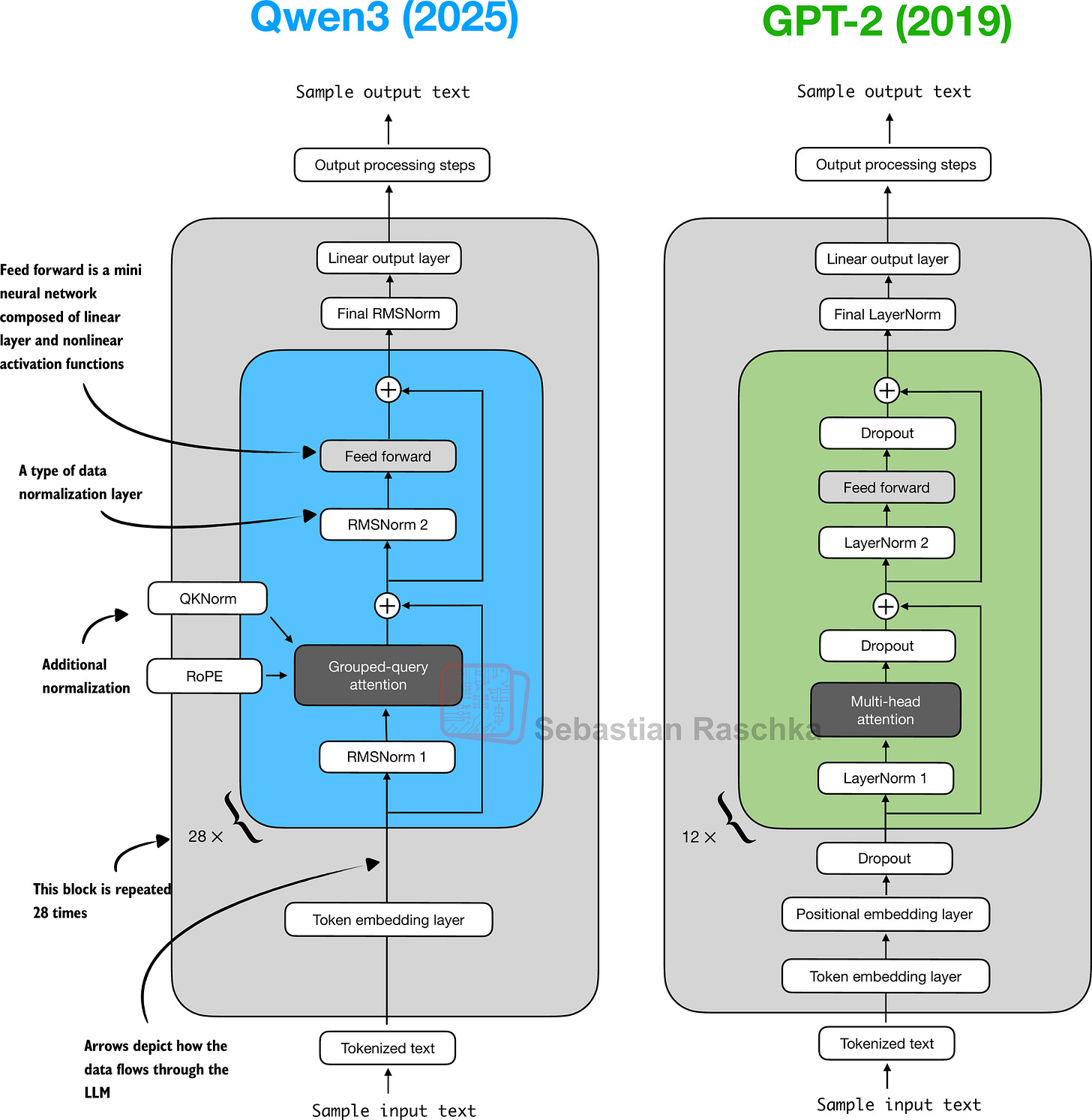
Figure 9 shows a side-by-side comparison between Qwen3 and GPT-2. 

Figure 9: Architectural comparison between Qwen3 0.6B and the 127M parameter GPT-2 variant. Both models process text through embedding layers and stacked transformer blocks, but they differ in certain design choices.

As illustrated in Figure 9, Qwen3 and GPT-2 both build on the decoder submodule of the original transformer architecture. Yet, the design has matured in the years since GPT-2. But most of Qwen3’s changes are not unique to this model: they reflect common practices across many contemporary LLMs, as I previously discussed in my architecture comparison article.

For readers new to LLMs, I think that GPT-2 is still an excellent starting point. Its simpler design makes it easier to implement and understand before implementing more advanced variations like Qwen3.

In case you read my Build a Large Language Model From Scratch book (which implements GPT-2), the Qwen3 implementation in the next sections follows a similar style, so if you are already comfortable with GPT-2, I hope it will be an easy read.

4 Normalization Layers

In contrast to GPT-2, which used standard LayerNorm, the newer Qwen3 architecture replaces it with root mean square layer normalization (RMSNorm). This is a trend that has become increasingly common in recent model architectures.

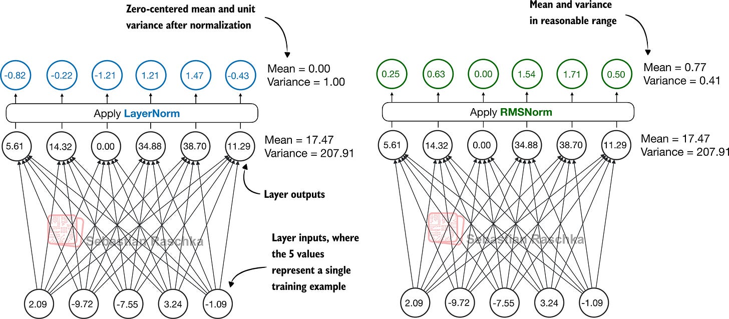
RMSNorm fulfills the same core function as LayerNorm: normalizing layer activations to stabilize and improve training. However, it simplifies the computation by removing the mean-centering step, as shown in Figure 10. This means that activations will still be normalized, but they are not centered at 0.

Figure 10: Comparison of LayerNorm and RMSNorm. LayerNorm (left) normalizes activations so that their average value (mean) is exactly zero and their spread (variance) is exactly one. RMSNorm (right) instead scales activations based on their root mean square, which does not enforce zero mean or unit variance, but still keeps the mean and variance within a reasonable range for stable training.

As we can see in Figure 10, both LayerNorm and RMSNorm scale the layer outputs to be in a reasonable range.

LayerNorm subtracts the mean and divides by the standard deviation such that the layer outputs have a zero mean and unit variance (variance of one and standard deviation of one), which results in favorable properties, in terms of gradient values, for stable training.

RMSNorm divides the inputs by the root mean square. This scales activations to a comparable magnitude without enforcing zero mean or unit variance. In this particular example shown in Figure 10, the mean is 0.77 and the variance is 0.41.

Both LayerNorm and RMSNorm stabilize activation scales and improve optimization; however, RMSNorm is often preferred in large-scale LLMs because it is computationally cheaper. Unlike LayerNorm, RMSNorm does not use a bias (shift) term by default, which reduces the number of trainable parameters. Moreover, RMSNorm reduces the expensive mean and variance computations to a single root-mean-square operation. This reduces the number of cross-feature reductions from two to one, which lowers communication overhead on GPUs and slightly improves training efficiency.

Below is how this looks like in code:       

import torch.nn as nn

class RMSNorm(nn.Module):

def __init__(
    self,
    emb_dim,
    eps=1e-6,
    bias=False,
    qwen3_compatible=True,
):
    super().__init__()
    self.eps = eps
    self.qwen3_compatible = qwen3_compatible
    self.scale = nn.Parameter(torch.ones(emb_dim))
    self.shift = (
        nn.Parameter(torch.zeros(emb_dim)) if bias
        else None
    )

    def forward(self, x):         input_dtype = x.dtype

        if self.qwen3_compatible:             x = x.to(torch.float32)

        variance = x.pow(2).mean(dim=-1, keepdim=True)         norm_x = x * torch.rsqrt(variance + self.eps)         norm_x = norm_x * self.scale

        if self.shift is not None:             norm_x = norm_x + self.shift

        return norm_x.to(input_dtype)

Note that, for brevity, this article does not provide detailed code walkthroughs for each LLM component. Instead, in section 9 (Main Model Class), we will integrate all components into the Qwen3Model class, load the pre-trained weights into it, and then use this model to generate text in section 12 (Using the Model).

While you can copy & paste the code into your editor or retype it (for a better learning experience), all the code examples are also available here on GitHub. In particular, see the:

standalone-qwen3-plus-kvcache.ipynb notebook for the dense model;

standalone-qwen3-moe-plus-kvcache.ipynb notebook for the MoE variant.

5 Feed Forward Module

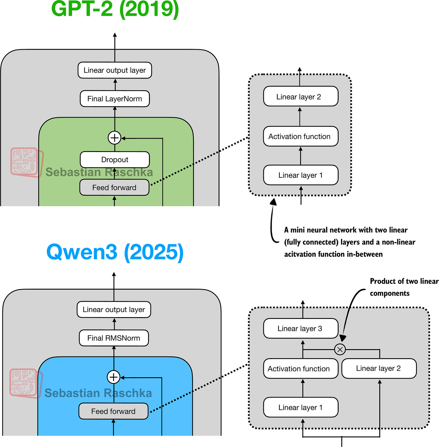
The feed forward module (a small multi-layer perceptron) is replaced with a gated linear unit (GLU) variant, introduced in a 2020 paper. In this design, the standard two fully connected layers are replaced by three, as shown in Figure 11.

Figure 11: In GPT-2 (top), the feed forward module consists of two fully connected (linear) layers separated by a non-linear activation function. In Qwen3 (bottom), this module is replaced with a gated linear unit (GLU) variant, which adds a third linear layer and multiplies its output elementwise with the activated output of the second linear layer.

Qwen3’s feed forward module (Figure 12) can be implemented as shown below:

class FeedForward(nn.Module): def init(self, cfg): super().__init__() self.fc1 = nn.Linear( cfg[“emb_dim”], cfg[“hidden_dim”], dtype=cfg[“dtype”], bias=False ) self.fc2 = nn.Linear( cfg[“emb_dim”], cfg[“hidden_dim”], dtype=cfg[“dtype”], bias=False ) self.fc3 = nn.Linear( cfg[“hidden_dim”], cfg[“emb_dim”], dtype=cfg[“dtype”], bias=False )

def forward(self, x):
    x_fc1 = self.fc1(x)
    x_fc2 = self.fc2(x)
    
    # The non-linear activation function here is a SiLU function,           
    # which will be discussed later
    x = nn.functional.silu(x_fc1) * x_fc2
    return self.fc3(x)

At first glance, it might seem that the GLU feed forward variant used in Qwen3 should outperform the standard feed forward variant in GPT-2, simply because it adds an extra linear layer (three instead of two) and therefore appears to have more parameters.

However, this intuition is misleading. In practice, the fc1 and fc2 layers in the GLU variant are each half the width of the fc1 layer in a standard feed forward module, and in practice, it has fewer parameters.

To illustrate this with a concrete example, suppose the input dimension to the “Linear layer 1” in Figure 12 is 1024. This corresponds to cfg[“emb_dim”] in the previous code. The output dimension of fc1 is 3,072 (cfg[“hidden_dim”]). Note that these are the actual numbers used in the Qwen3 0.6B variant. In this case, we have the following parameter counts for the GLU variant in the previous code:

fc1: 1024 × 3,072 = 3,145,728  

fc2: 1024 × 3,072 = 3,145,728 

fc3: 1024 × 3,072 = 3,145,728  

Total: 3 × 3,145,728 = 9,437,184 parameters

If we assume that fc1 in this GLU variant has half the width as would be typically chosen for an fc1 in a standard feed forward module, the parameter counts of the standard feed forward module would be as follows:

fc1: 1024 × 2×3,072 = 6,291,456  

fc2: 1024 × 2×3,072 = 6,291,456 

Total: 2 × 6,291,456 = 12,582,912 parameters

While GLU variants usually have fewer parameters than regular feed forward modules, they perform better. The improvement comes from the additional multiplicative interaction introduced by the gating mechanism, activation(x_fc1) * x_fc2, which increases the model’s expressivity. This is similar to how deeper, slimmer networks can outperform shallower, wider ones, given proper training.

Before we proceed to the next section, there is one more thing to address. Note that the feed forward module shown in Figure 12 contains an element labeled as “Activation function,” whereas we used a nn.functional.silu activation as a concrete example in the previous code sample.

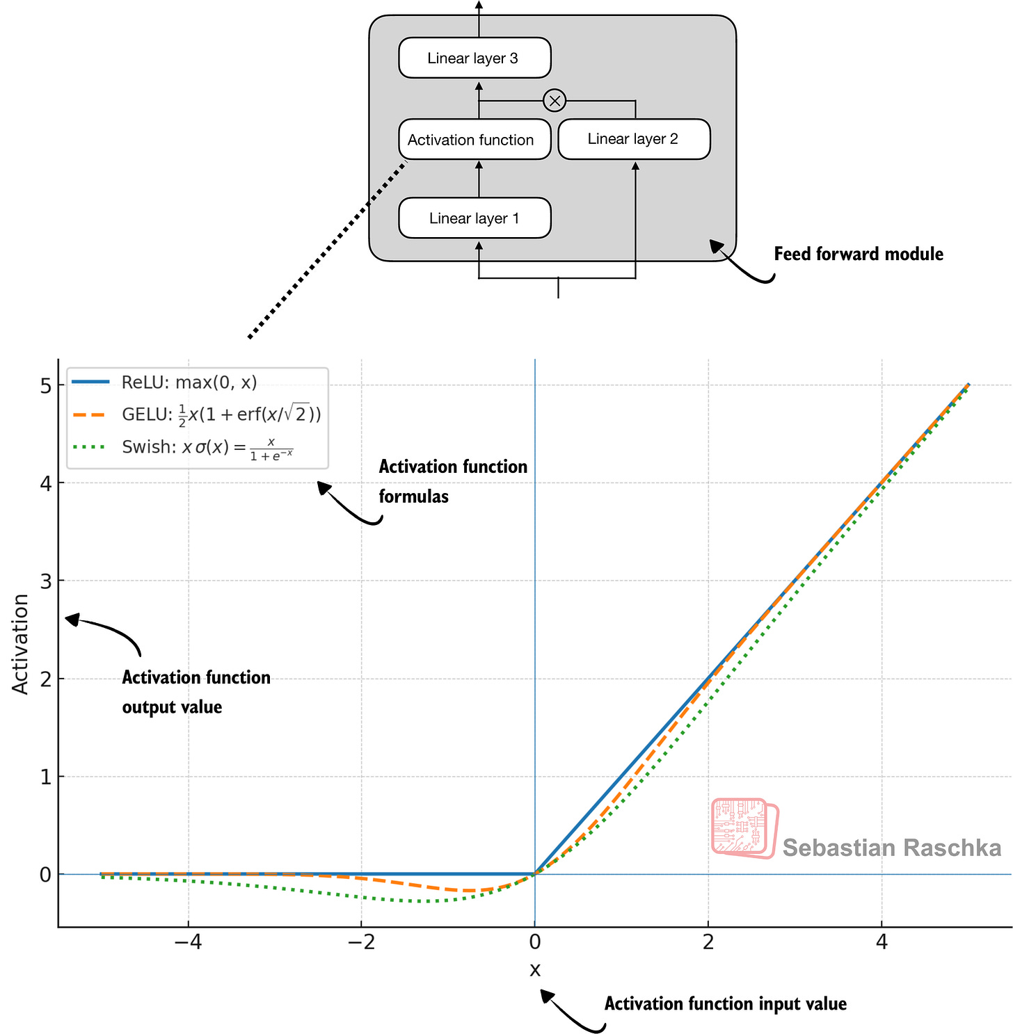
Historically, activation functions were a hot topic of debate until the deep learning community largely converged on the rectified linear unit (ReLU) more than a decade ago. ReLU is simple and computationally cheap, but it has a sharp kink at zero. This motivated researchers to explore smoother functions such as the Gaussian error linear unit (GELU) and the sigmoid linear unit (SiLU), as shown in Figure 12.

Figure 12: Different activation functions that can be used in a feed forward module (neural network). GELU and SiLU (Swish) offer smooth alternatives to ReLU, which has a sharp kink at input zero.

GELU involves the Gaussian cumulative distribution function (CDF). Computing this CDF is slow because it uses piecewise logic and exponentials, which makes it hard to write fused, optimized GPU kernels (although a tanh approximation exists that uses cheaper operations and runs faster with near-identical results).

In short, while GELU produces smooth activation curves, it is overall computationally more expensive than simpler functions. 

Newer models have largely replaced GELU with the SiLU (also known as Swish) function, which smoothly suppresses large negative inputs toward ~0 and is approximately linear for large positive inputs, as shown in Figure 12.

SiLU has a similar smoothness, but it is slightly cheaper to compute than GELU and offers comparable modeling performance. In practice, SiLU is now used in most architectures, while GELU remains in use in only some models, such as Google’s Gemma open-weight LLM. In the implementation of the feed forward module in the previous FeedForward code, this SiLU function is called via nn.functional.silu. The feed forward module (FeedForward) is also often called SwiGLU, an abbreviation that is derived from the terms Swish and GLU.

6 Rotary Position Embeddings (RoPE)

In transformer-based LLMs, positional encoding is necessary because of the attention mechanism. By default, attention treats the input tokens as if they have no order. In the original GPT architecture, absolute positional embeddings addressed this by adding a learned embedding vector for each position in the sequence, which is then added to the token embeddings.

RoPE (short for rotary position embeddings) introduced a different approach: instead of adding position information as separate embeddings, it encodes position information by rotating the query and key vectors in the attention mechanism (section 7) in a way that depends on each token’s position. RoPE is an elegant idea, but also a long topic in itself. Interested readers can find more information in the original RoPE paper. (While first introduced in 2021, RoPE became widely adopted with the release of the original Llama model in 2023 and has since become a staple in modern LLMs, so it is not unique to Qwen3.)

RoPE can be implemented in two mathematically equivalent ways: the interleaved form, which pairs adjacent dimensions for rotation, or in a two-halves form, which splits the dimension into cosine and sine halves for convenience. The code below implements the two-halves variant, which can be easier to read.          

import torch

def compute_rope_params( head_dim, theta_base=10_000, context_length=4096, dtype=torch.float32, ): assert head_dim % 2 == 0, “Embedding dim must be even”

inv_freq = 1.0 / (
    theta_base
    ** (
        torch.arange(0, head_dim, 2, dtype=dtype)[: head_dim // 2]
        .float()
        / head_dim
    )
)

positions = torch.arange(context_length, dtype=dtype)
angles = positions[:, None] * inv_freq[None, :]
angles = torch.cat([angles, angles], dim=1)

cos = torch.cos(angles)
sin = torch.sin(angles)

return cos, sin

def apply_rope(x, cos, sin, offset=0):

batch_size, num_heads, seq_len, head_dim = x.shape
assert head_dim % 2 == 0, "Head dimension must be even"

# Split x into first half and second half
x1 = x[..., : head_dim // 2]  # First half
x2 = x[..., head_dim // 2:]  # Second half


cos = cos[offset:offset + seq_len, :].unsqueeze(0).unsqueeze(0)
sin = sin[offset:offset + seq_len, :].unsqueeze(0).unsqueeze(0)
# Shape after:  (1, 1, seq_len, head_dim)

rotated = torch.cat((-x2, x1), dim=-1)
x_rotated = (x * cos) + (rotated * sin)


return x_rotated.to(dtype=x.dtype)

Later, in the Qwen3Model class implementation (section 9), we will compute and store the cos and sin values:

cos, sin = compute_rope_params( head_dim=head_dim, theta_base=cfg[“rope_base”], context_length=cfg[“context_length”] )

Then, inside the grouped query attention module (section 7) inside each transformer block, we apply the rotation to the queries and keys:

queries = apply_rope(queries, cos, sin, offset=start_pos) keys = apply_rope(keys_new, cos, sin, offset=start_pos)

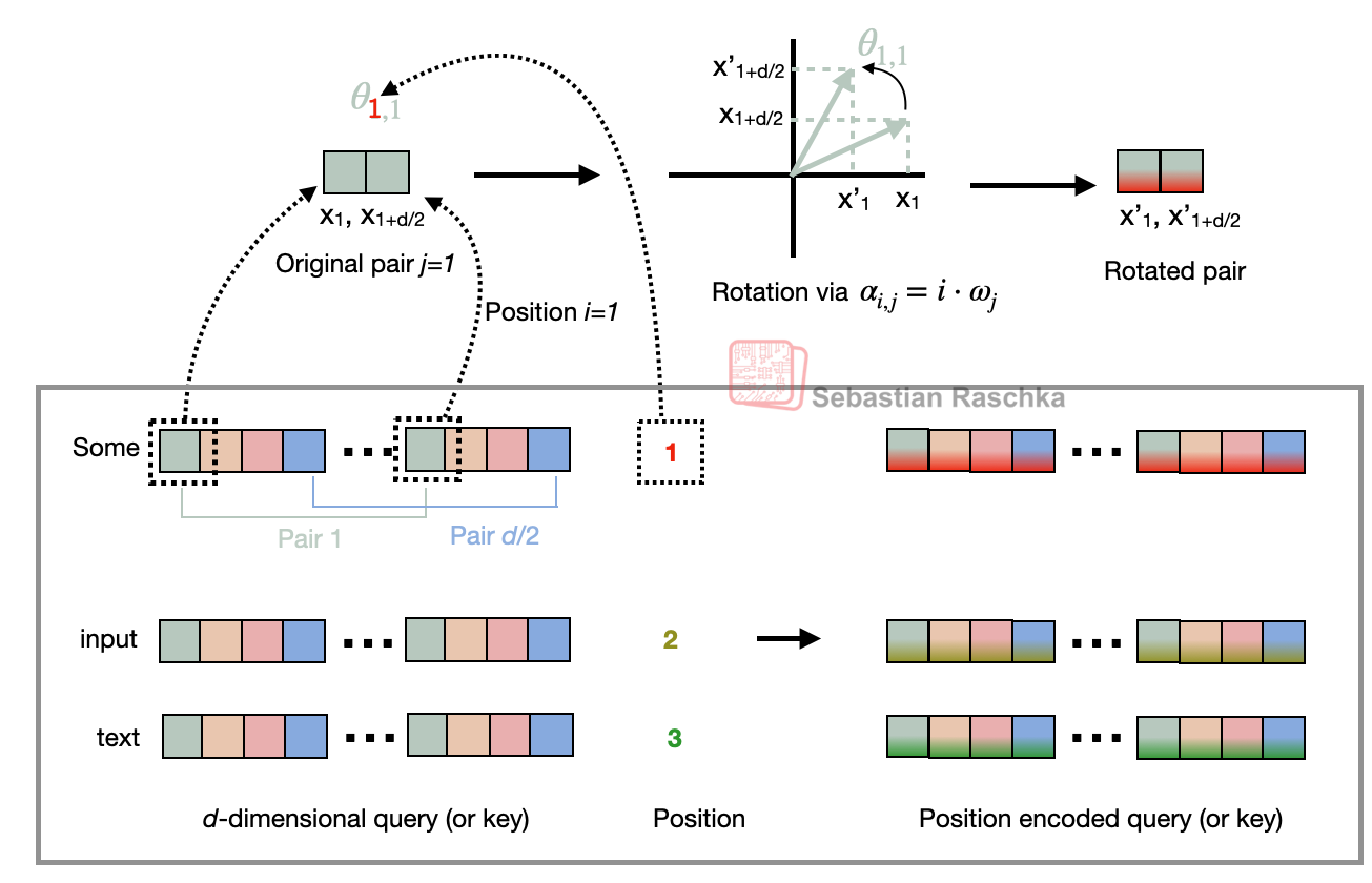
Let’s briefly go over what’s happening in the two functions (compute_rope_params and apply_rope) that implement the RoPE two-halves variant, using the same indices as in the figure.

Inside the apply_rope function, we take a d-dimensional query or key (with even d) for each attention head and pair across the two halves:

𝑥

[ 𝑥 1 , … , 𝑥 𝑑] ∈ 𝑅 𝑑 , pairs  ( 𝑥 𝑗 , 𝑥 𝑗 + 𝑑 / 2 )  for  𝑗 = 1 , … , 𝑑 2 .

Each pair

( 𝑥 𝑗 , 𝑥 𝑗 + 𝑑 / 2 )

is treated as a 2D coordinate that is rotated by an angle depending on the token position i, as illustrated in Figure 13.

Figure 13: Illustration of the RoPE two-halves variant. Here, it shows how a position pair in the query (or key) vector is rotated via a rotation angle α_{i,j}, which is based on a position i and a frequency constant ω_j. The figure is inspired by Figure 1 in the original RoPE paper.

The rotation depicted in Figure 13 works as follows, in 3 main steps.

Step 1: Construct the frequency basis

In compute_rope_params we define the vector inv_freq of length d/2:

𝜔 𝑗 = inv_freq 𝑗 = 𝜃 base − 2 ( 𝑗 − 1 ) 𝑑 , 𝑗 = 1 , … , 𝑑 2 .

(Note that the code uses 0-based indexing instead of 1-based indexing due to how Python and PyTorch work.)

The base constant, θ_base (theta_base) is a hyperparameter set to a default value of 10,000 in the code signature above. Qwen3 uses θ_base = 1,000,000 to enable much longer contexts than the classic 10,000 setting.

Step 2: Compute angles for each position

For every token position i, we build the angle table for angles α_{i,j}:

𝛼 𝑖 , 𝑗 = 𝑖 ⋅ inv_freq 𝑗 ,

and then precompute

cos 𝑖 , 𝑗 = cos ⁡ ( 𝛼 𝑖 , 𝑗 ) , sin 𝑖 , 𝑗 = sin ⁡ ( 𝛼 𝑖 , 𝑗 ) .

Step 3: Rotate the two halves

Given a pair

( 𝑥 𝑗 , 𝑥 𝑗 + 𝑑 / 2 )

at token position i, we can then rotate it by the corresponding entry from the cos/sin tables:

𝑥 𝑗 ′

= 𝑥 𝑗 cos 𝑖 , 𝑗 − 𝑥 𝑗 + 𝑑 / 2 sin 𝑖 , 𝑗 ,

𝑥 𝑗 + 𝑑 / 2 ′

= 𝑥 𝑗 sin 𝑖 , 𝑗 + 𝑥 𝑗 + 𝑑 / 2 cos 𝑖 , 𝑗 .

Equivalently, for each j-th pair, we can compute the rotated pair using a rotation matrix:

[ 𝑥 𝑗 ′

𝑥 𝑗 + 𝑑 / 2 ′ ] = [ cos 𝑖 , 𝑗

− sin 𝑖 , 𝑗

sin 𝑖 , 𝑗

  cos 𝑖 , 𝑗 ] [ 𝑥 𝑗

𝑥 𝑗 + 𝑑 / 2 ] .

Note that we look at a single head for simplicity. However, RoPE is applied identically to every attention head: we compute one cos/sin table for shape (context_length, head_dim) and broadcast it across the num_heads dimension for both queries and keys (including KV-groups in GQA).

7 Grouped Query Attention (GQA)

Grouped query attention (GQA) has become the standard, more compute- and parameter-efficient alternative to the original multi-head attention (MHA) mechanism.

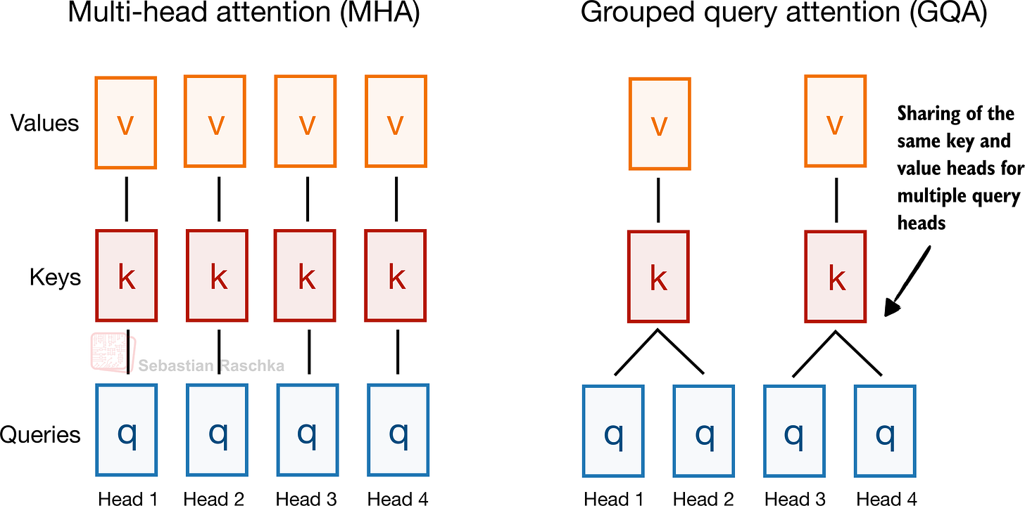
Unlike MHA, where each head also has its own set of keys and values, to reduce memory usage, GQA groups multiple heads to share the same key and value projections, as shown in Figure 14.

Figure 14: A comparison between MHA and GQA. Here, the group size is 2, where a key and value pair is shared among 2 queries.

So, the core idea behind GQA, shown in Figure 14, is to reduce the number of key and value heads by sharing them across multiple query heads. This (1) lowers the model’s parameter count and (2) reduces the memory bandwidth usage for key and value tensors during inference since fewer keys and values need to be stored and retrieved from the KV cache (section 10).

While GQA is primarily a computational efficiency workaround for MHA, ablation studies (as presented in the original GQA paper) show that it performs comparably to standard MHA in terms of LLM modeling performance.

The code below implements the GQA mechanism with KV cache support.

class GroupedQueryAttention(nn.Module): def init(self, d_in, num_heads, num_kv_groups, head_dim=None, qk_norm=False, dtype=None): super().__init__() assert num_heads % num_kv_groups == 0

    self.num_heads = num_heads
    self.num_kv_groups = num_kv_groups
    self.group_size = num_heads // num_kv_groups

    if head_dim is None:
        assert d_in % num_heads == 0
        head_dim = d_in // num_heads

    self.head_dim = head_dim
    self.d_out = num_heads * head_dim

    self.W_query = nn.Linear(
        d_in, self.d_out, bias=False, dtype=dtype
    )
    self.W_key = nn.Linear(
        d_in, num_kv_groups * head_dim, bias=False,dtype=dtype
    )
    self.W_value = nn.Linear(
        d_in, num_kv_groups * head_dim, bias=False, dtype=dtype
    )

    self.out_proj = nn.Linear(
        self.d_out, d_in, bias=False, dtype=dtype
    )

    if qk_norm:
        self.q_norm = RMSNorm(head_dim, eps=1e-6)
        self.k_norm = RMSNorm(head_dim, eps=1e-6)
    else:
        self.q_norm = self.k_norm = None

def forward(self, x, mask, cos, sin, start_pos=0, cache=None):
    b, num_tokens, _ = x.shape

    queries = self.W_query(x)  # (b, n_tok, n_heads * head_dim)
    keys = self.W_key(x) (b,   # (b, n_tok, n_kv_groups * head_dim)
    values = self.W_value(x)   # (b, n_tok, n_kv_groups * head_dim)

    queries = queries.view(b, num_tokens, self.num_heads,
                           self.head_dim).transpose(1, 2)
    keys_new = keys.view(b, num_tokens, self.num_kv_groups,
                         self.head_dim).transpose(1, 2)
    values_new = values.view(b, num_tokens, self.num_kv_groups,
                             self.head_dim).transpose(1, 2)

    if self.q_norm:
        queries = self.q_norm(queries)
    if self.k_norm:
        keys_new = self.k_norm(keys_new)

    queries = apply_rope(queries, cos, sin, offset=start_pos)
    keys_new = apply_rope(keys_new, cos, sin, offset=start_pos)

    if cache is not None:
        prev_k, prev_v = cache
        keys = torch.cat([prev_k, keys_new], dim=2)
        values = torch.cat([prev_v, values_new], dim=2)
    else:
        start_pos = 0  # Reset RoPE
        keys, values = keys_new, values_new            
    next_cache = (keys, values)

    # Expand K and V to match number of heads
    keys = keys.repeat_interleave(  
        self.group_size, dim=1
    )
    values = values.repeat_interleave(
        self.group_size, dim=1
    )

    attn_scores = queries @ keys.transpose(2, 3)
    attn_scores = attn_scores.masked_fill(mask, -torch.inf)
    attn_weights = torch.softmax(
        attn_scores / self.head_dim**0.5, dim=-1

       

You may have noticed that the GQA mechanism in the code above also includes a qk_norm parameter. This is not part of the standard GQA design. When qk_norm=True, an additional Query/Key-RMSNorm-based normalization, called QKNorm, is applied to both the queries and keys, which is a technique used in Qwen3. As discussed earlier in the RMSNorm section (section 4), QKNorm helps improve training stability.

8 The Transformer Block

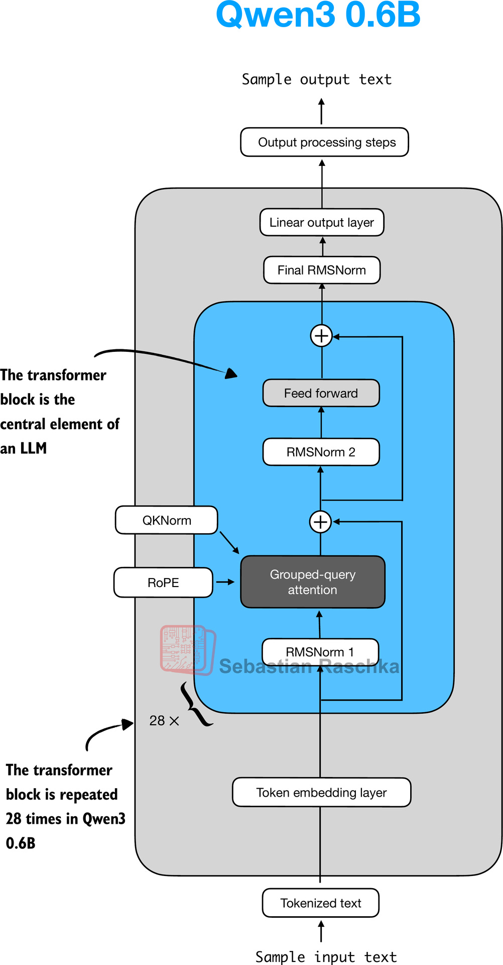
The transformer block is the central component of an LLM, which combines all the individual elements covered in this appendix so far. As shown in Figure 15, it is repeated multiple times; in the 0.6-billion-parameter version of Qwen3, it is repeated 28 times.

Figure 15: The Structure of the transformer block in Qwen3. Each block includes RMSNorm, RoPE, masked grouped-query attention, and a feed-forward module, and is repeated 28 times in the 0.6B-parameter model.

The following code implements the transformer block:

class TransformerBlock(nn.Module): def init(self, cfg): super().__init__() self.att = GroupedQueryAttention( d_in=cfg[“emb_dim”], num_heads=cfg[“n_heads”], head_dim=cfg[“head_dim”], num_kv_groups=cfg[“n_kv_groups”], qk_norm=cfg[“qk_norm”], dtype=cfg[“dtype”] ) self.ff = FeedForward(cfg) self.norm1 = RMSNorm(cfg[“emb_dim”], eps=1e-6) self.norm2 = RMSNorm(cfg[“emb_dim”], eps=1e-6)

def forward(self, x, mask, cos, sin, start_pos=0, cache=None):
    shortcut = x
    x = self.norm1(x)
    x, next_cache = self.att(
        x, mask, cos, sin, start_pos=start_pos,cache=cache
    )  # (batch_size, num_tokens, emb_size)
    x = x + shortcut

    shortcut = x
    x = self.norm2(x)
    x = self.ff(x)
    x = x + shortcut

    return x, next_cache 

As we can see, the transformer block simply connects various elements we implemented in previous sections.

9 Main Model Class

In this section, we will define the Qwen3Model class, where the previously implemented transformer block sits at the heart of the LLM.     

class Qwen3Model(nn.Module): def init(self, cfg): super().__init__()

    # Main model parameters
    self.tok_emb = nn.Embedding(cfg["vocab_size"], cfg["emb_dim"],
                                dtype=cfg["dtype"])

    self.trf_blocks = nn.ModuleList(
        [TransformerBlock(cfg) for _ in range(cfg["n_layers"])]
    )
    self.final_norm = RMSNorm(cfg["emb_dim"])
    self.out_head = nn.Linear(
        cfg["emb_dim"], cfg["vocab_size"],
        bias=False, dtype=cfg["dtype"]
    )

    # Reusable utilities
    if cfg["head_dim"] is None:
        head_dim = cfg["emb_dim"] // cfg["n_heads"]
    else:
        head_dim = cfg["head_dim"]
    cos, sin = compute_rope_params(
        head_dim=head_dim,
        theta_base=cfg["rope_base"],
        context_length=cfg["context_length"]
    )
    self.register_buffer("cos", cos, persistent=False)
    self.register_buffer("sin", sin, persistent=False)
    self.cfg = cfg
    self.current_pos = 0  # Track current position in KV cache

def forward(self, in_idx, cache=None):
    # Forward pass
    tok_embeds = self.tok_emb(in_idx)
    x = tok_embeds

    num_tokens = x.shape[1]
    if cache is not None:
        pos_start = self.current_pos
        pos_end = pos_start + num_tokens
        self.current_pos = pos_end
        mask = torch.triu(
            torch.ones(
                pos_end, pos_end, device=x.device, dtype=torch.bool
            ),
            diagonal=1
        )[pos_start:pos_end, :pos_end]
    else:
        pos_start = 0  # Not strictly necessary but helps torch.compile
        mask = torch.triu(
            torch.ones(num_tokens, num_tokens, device=x.device,
                       dtype=torch.bool),
            diagonal=1
        )
    # Prefill (no cache): mask starts as (num_tokens, num_tokens)
    # Cached decoding: mask starts as (num_tokens, prev_k_number_tokens + num_tokens)
    #
    # We add two leading dimensions so the mask becomes
    # (1, 1, num_tokens, num_tokens) during prefill and
    # (1, 1, num_tokens, total_key_tokens) during cached decoding.
    # These extra dimensions let PyTorch broadcast the same mask
    # across all batches and attention heads when applying it to
    # attn_scores of shape (batch, num_heads, num_tokens, total_key_tokens).
    mask = mask[None, None, :, :]

    for i, block in enumerate(self.trf_blocks):
        blk_cache = cache.get(i) if cache else None
        x, new_blk_cache = block(x, mask, self.cos, self.sin,
                                 start_pos=pos_start,
                                 cache=blk_cache)
        if cache is not None:
            cache.update(i, new_blk_cache)

    x = self.final_norm(x)
    logits = self.out_head(x.to(self.cfg["dtype"]))
    return logits

def reset_kv_cache(self):
    self.current_pos = 0

Since we already have all the main ingredients, the Qwen3Model class only adds a few more components around the transformer block, namely the embedding and output layers (including one more RMSNorm layer). However, the code may appear somewhat complicated, which is due to the KV cache option.

As discussed in my earlier Understanding and Coding the KV Cache in LLMs from Scratch article, the KV cache can speed up the text generation process, but it is a topic outside the scope of this book.

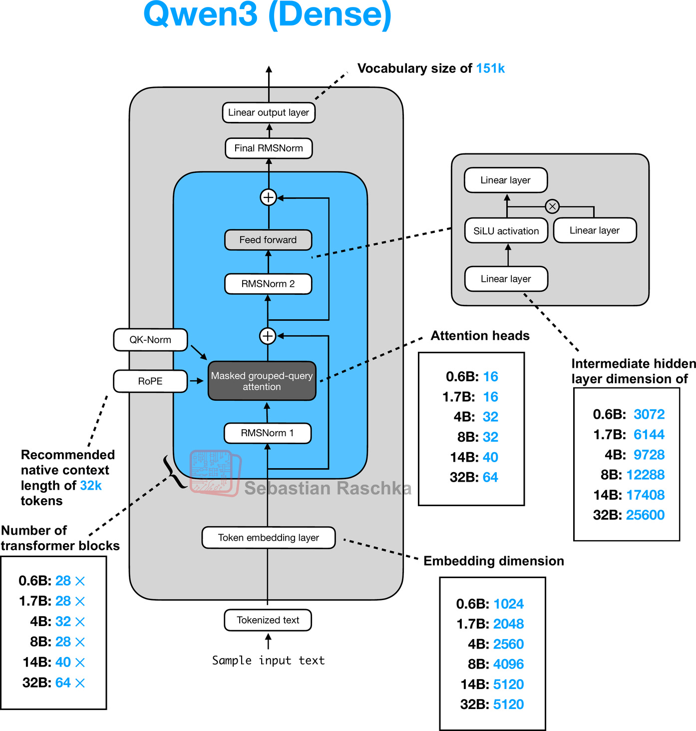
Note that the Qwen3Model class supports various model sizes. The overall architecture along with the differences for each size, is shown in Figure 16 below.

Figure 16: Architecture of the Qwen3 0.6B model. The model consists of a token embedding layer followed by 28 transformer blocks, each containing RMSNorm, RoPE, QKNorm, masked grouped-query attention with 16 heads, and a feed-forward module with an intermediate size of 3,072.

To use the 0.6B model via the Qwen3Model class, we can define the following configuration in that we provide as input (cfg=QWEN_CONFIG) upon instantiating a new Qwen3Model instance.                      

CHOOSE_MODEL = “0.6B”

if CHOOSE_MODEL == “0.6B”: QWEN3_CONFIG = { “vocab_size”: 151_936, # Vocabulary size “context_length”: 40_960, # Context length that was used to train the model “emb_dim”: 1024, # Embedding dimension “n_heads”: 16, # Number of attention heads “n_layers”: 28, # Number of layers “hidden_dim”: 3072, # Size of the intermediate dimension in FeedForward “head_dim”: 128, # Size of the heads in GQA “qk_norm”: True, # Whether to normalize queries and keys in GQA “n_kv_groups”: 8, # Key-Value groups for grouped-query attention “rope_base”: 1_000_000.0, # The base in RoPE’s “theta” “dtype”: torch.bfloat16, # Lower-precision dtype to reduce memory usage }

elif CHOOSE_MODEL == “1.7B”: QWEN3_CONFIG = { “vocab_size”: 151_936, “context_length”: 40_960, “emb_dim”: 2048, # 2x larger than above “n_heads”: 16, “n_layers”: 28, “hidden_dim”: 6144, # 2x larger than above “head_dim”: 128, “qk_norm”: True, “n_kv_groups”: 8, “rope_base”: 1_000_000.0, “dtype”: torch.bfloat16, }

elif CHOOSE_MODEL == “4B”: QWEN3_CONFIG = { “vocab_size”: 151_936, “context_length”: 40_960, “emb_dim”: 2560, # 25% larger than above “n_heads”: 32, # 2x larger than above “n_layers”: 36, # 29% larger than above “hidden_dim”: 9728, # ~3x larger than above “head_dim”: 128, “qk_norm”: True, “n_kv_groups”: 8, “rope_base”: 1_000_000.0, “dtype”: torch.bfloat16, }

elif CHOOSE_MODEL == “8B”: QWEN3_CONFIG = { “vocab_size”: 151_936, “context_length”: 40_960, “emb_dim”: 4096, # 60% larger than above “n_heads”: 32, “n_layers”: 36,
“hidden_dim”: 12288, # 26% larger than above “head_dim”: 128, “qk_norm”: True, “n_kv_groups”: 8, “rope_base”: 1_000_000.0, “dtype”: torch.bfloat16, }

elif CHOOSE_MODEL == “14B”: QWEN3_CONFIG = { “vocab_size”: 151_936, “context_length”: 40_960, “emb_dim”: 5120, # 25% larger than above “n_heads”: 40, # 25% larger than above “n_layers”: 40, # 11% larger than above “hidden_dim”: 17408, # 42% larger than above “head_dim”: 128, “qk_norm”: True, “n_kv_groups”: 8, “rope_base”: 1_000_000.0, “dtype”: torch.bfloat16, }

elif CHOOSE_MODEL == “32B”: QWEN3_CONFIG = { “vocab_size”: 151_936, “context_length”: 40_960, “emb_dim”: 5120,
“n_heads”: 64, # 60% larger than above “n_layers”: 64, # 60% larger than above “hidden_dim”: 25600, # 47% larger than above “head_dim”: 128, “qk_norm”: True, “n_kv_groups”: 8, “rope_base”: 1_000_000.0, “dtype”: torch.bfloat16, }

else: raise ValueError(f”{CHOOSE_MODEL} is not supported.”)

We can then initiate the model as follows:

model = Qwen3Model(QWEN3_CONFIG)

10 KV Cache

The KV-cache-related heavy-lifting is mostly done in the Qwen3Model (section 9) and GroupedQueryAttention (section 7) code. Since the article on KV caching was so recent, I hope you don’t mind me just linking it here for reference instead of providing a longer explanation.

The KVCache, shown below, stores the key-value pairs themselves during text generation, which results in the speedup we experienced when enabling KV caching.

class KVCache: def init(self, n_layers): self.cache = [None] * n_layers

def get(self, layer_idx):
    return self.cache[layer_idx]

def update(self, layer_idx, value):
    self.cache[layer_idx] = value

def get_all(self):
    return self.cache

def reset(self):
    for i in range(len(self.cache)):
        self.cache[i] = None

The KVCache class is used inside the generate_text_basic_cache function that we implemented in chapter 2.

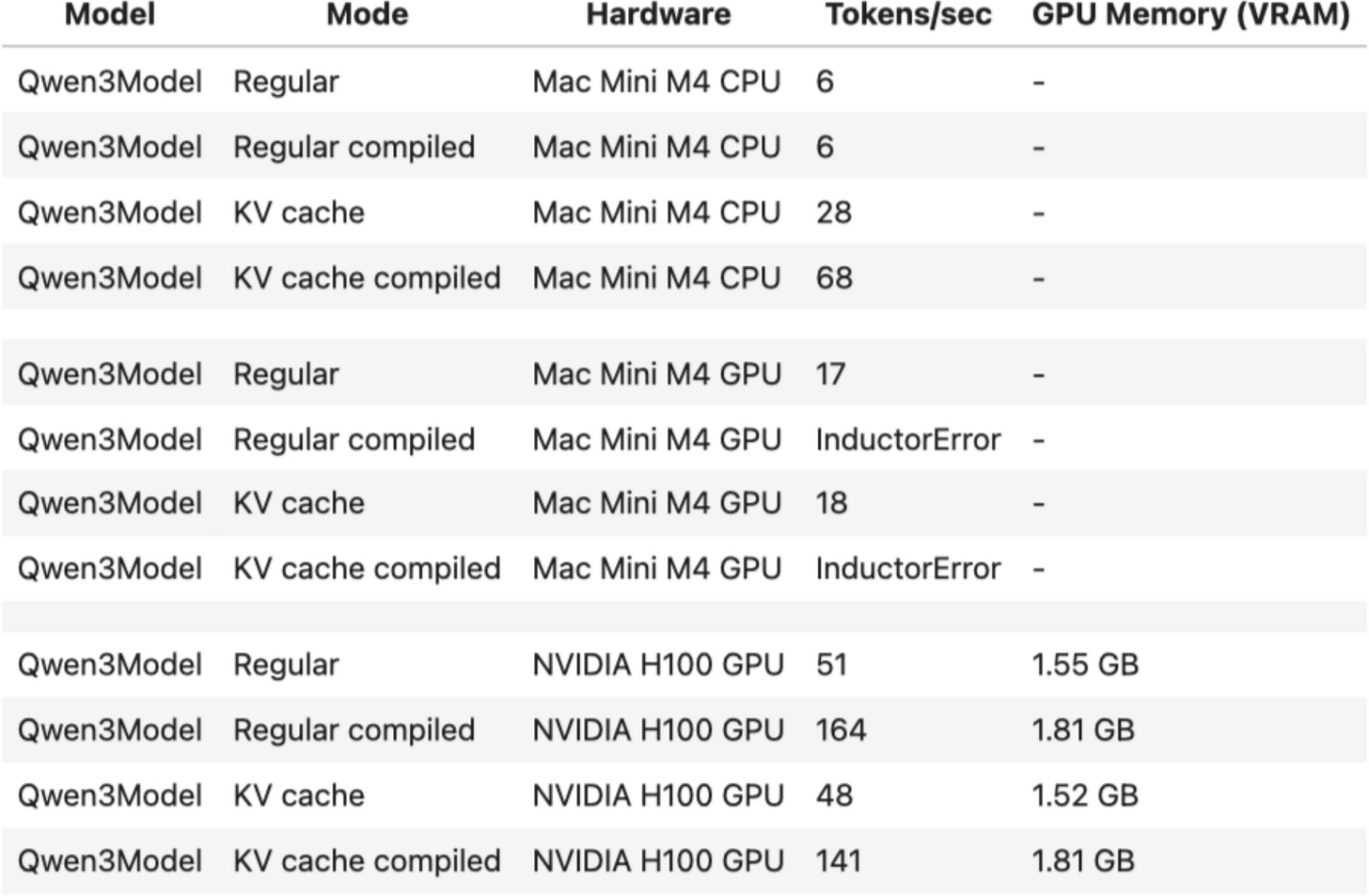
The speed-up is summarized in the table below for the 0.6B model in PyTorch 2.7.1.

Figure 17: Speed-comparison between a regular and KV cache implementation of Qwen3 0.6B.

11 Tokenizer

The tokenizer code is somewhat complicated, as it supports a variety of special tokens, in addition to the base model and the so-called “Thinking” model variant of Qwen3, which is a reasoning model. The full reimplementation of the tokenizer is shown below.

from pathlib import Path import re from tokenizers import Tokenizer

class Qwen3Tokenizer: _SPECIALS = [ “<|endoftext|>”, “<|im_start|>”, “<|im_end|>”, “<|object_ref_start|>”, “<|object_ref_end|>”, “<|box_start|>”, “<|box_end|>”, “<|quad_start|>”, “<|quad_end|>”, “<|vision_start|>”, “<|vision_end|>”, “<|vision_pad|>”, “<|image_pad|>”, “<|video_pad|>”, ] _SPLIT_RE = re.compile(r”(<|[^>]+?|>)“)

def __init__(self,
             tokenizer_file_path="tokenizer-base.json",
             apply_chat_template=False,
             add_generation_prompt=False,
             add_thinking=False):

    self.apply_chat_template = apply_chat_template
    self.add_generation_prompt = add_generation_prompt
    self.add_thinking = add_thinking

    tok_path = Path(tokenizer_file_path)
    if not tok_path.is_file():
        raise FileNotFoundError(
            f"Tokenizer file '{tok_path}' not found. "
        )

    self._tok = Tokenizer.from_file(str(tok_path))
    self._special_to_id = {t: self._tok.token_to_id(t) 
                           for t in self._SPECIALS}

    self.pad_token = "<|endoftext|>"
    self.pad_token_id = self._special_to_id.get(self.pad_token)

    # Match HF behavior: chat model: <|im_end|>, base model: <|endoftext|>
    f = tok_path.name.lower()    
    if "base" in f and "reasoning" not in f:
        self.eos_token = "<|endoftext|>"
    else:                              
        self.eos_token = "<|im_end|>"
    self.eos_token_id = self._special_to_id.get(self.eos_token)

def encode(self, prompt, chat_wrapped=None):
    if chat_wrapped is None:
        chat_wrapped = self.apply_chat_template

    stripped = prompt.strip()
    if stripped in self._special_to_id and "\n" not in stripped:
        return [self._special_to_id[stripped]]

    if chat_wrapped:
        prompt = self._wrap_chat(prompt)

    ids = []
    for part in filter(None, self._SPLIT_RE.split(prompt)):
        if part in self._special_to_id:
            ids.append(self._special_to_id[part])
        else:
            ids.extend(self._tok.encode(part).ids)
    return ids

def decode(self, token_ids):
    return self._tok.decode(token_ids, skip_special_tokens=False)

def _wrap_chat(self, user_msg):
    s = f"<|im_start|>user\n{user_msg}<|im_end|>\n"
    if self.add_generation_prompt:
        s += "<|im_start|>assistant"
        if self.add_thinking:
            s += "\n" #insert no <think> tag, just a new line
        else:
            s += "\n<think>\n\n</think>\n\n"
    return s

Note that my Qwen3Tokenizer reimplementation may appear somewhat complicated, as it aims to replicate the behavior of the official tokenizer released by the Qwen3 team in the Hugging Face transformers library (I have unit tests that check for parity).

At first glance, it appears to have a few quirks. For example, when add_thinking=True, no “” tokens are inserted (where is a newline character), and when add_thinking=False, these tokens are added. This is intentional because the non-base Qwen3 0.6B model is a hybrid that supports both reasoning (“thinking”) and standard modes. 

12 Using the Model

Let’s now instantiate and use the model to confirm that the code works by loading the pre-trained Qwen3 weights and using the model on a prompt

In section 9, we briefly talked about the model initialization via

model = Qwen3Model(QWEN3_CONFIG)

This code above initializes the model with random weights. Now, to load the official pre-trained weights into our architecture, we can define the following helper function:

def load_weights_into_qwen(model, param_config, params): def assign(left, right, tensor_name=“unknown”): if left.shape != right.shape: raise ValueError( f”Shape mismatch in tensor ” f”‘{tensor_name}’. Left: {left.shape}, ” f”Right: {right.shape}” ) return torch.nn.Parameter( right.clone().detach() if isinstance(right, torch.Tensor) else torch.tensor(right) )

model.tok_emb.weight = assign(
    model.tok_emb.weight,
    params["model.embed_tokens.weight"],
    "model.embed_tokens.weight"
)

for l in range(param_config["n_layers"]):
    block = model.trf_blocks[l]
    att = block.att

    # Q, K, V projections
    att.W_query.weight = assign(
        att.W_query.weight,
        params[f"model.layers.{l}.self_attn.q_proj.weight"],
        f"model.layers.{l}.self_attn.q_proj.weight"
    )
    att.W_key.weight = assign(
        att.W_key.weight,
        params[f"model.layers.{l}.self_attn.k_proj.weight"],
        f"model.layers.{l}.self_attn.k_proj.weight"
    )
    att.W_value.weight = assign(
        att.W_value.weight,
        params[f"model.layers.{l}.self_attn.v_proj.weight"],
        f"model.layers.{l}.self_attn.v_proj.weight"
    )

    # Output projection
    att.out_proj.weight = assign(
        att.out_proj.weight,
        params[f"model.layers.{l}.self_attn.o_proj.weight"],
        f"model.layers.{l}.self_attn.o_proj.weight"
    )

    # QK norms
    if hasattr(att, "q_norm") and att.q_norm is not None:
        att.q_norm.scale = assign(
            att.q_norm.scale,
            params[f"model.layers.{l}.self_attn.q_norm.weight"],
            f"model.layers.{l}.self_attn.q_norm.weight"
        )
    if hasattr(att, "k_norm") and att.k_norm is not None:
        att.k_norm.scale = assign(
            att.k_norm.scale,
            params[f"model.layers.{l}.self_attn.k_norm.weight"],
            f"model.layers.{l}.self_attn.k_norm.weight"
        )

    # Attention layernorm
    block.norm1.scale = assign(
        block.norm1.scale,
        params[f"model.layers.{l}.input_layernorm.weight"],
        f"model.layers.{l}.input_layernorm.weight"
    )

    # Feedforward weights
    block.ff.fc1.weight = assign(
        block.ff.fc1.weight,
        params[f"model.layers.{l}.mlp.gate_proj.weight"],
        f"model.layers.{l}.mlp.gate_proj.weight"
    )
    block.ff.fc2.weight = assign(
        block.ff.fc2.weight,
        params[f"model.layers.{l}.mlp.up_proj.weight"],
        f"model.layers.{l}.mlp.up_proj.weight"
    )
    block.ff.fc3.weight = assign(
        block.ff.fc3.weight,
        params[f"model.layers.{l}.mlp.down_proj.weight"],
        f"model.layers.{l}.mlp.down_proj.weight"
    )
    block.norm2.scale = assign(
        block.norm2.scale,
        params[f"model.layers.{l}.post_attention_layernorm.weight"],
        f"model.layers.{l}.post_attention_layernorm.weight"
    )

# Final normalization and output head
model.final_norm.scale = assign(
    model.final_norm.scale,
    params["model.norm.weight"],
    "model.norm.weight"
)

if "lm_head.weight" in params:
    model.out_head.weight = assign(
        model.out_head.weight,
        params["lm_head.weight"],
        "lm_head.weight"
    )
else:
    # Model uses weight tying
    print("Model uses weight tying.")
    model.out_head.weight = assign(
        model.out_head.weight,
        params["model.embed_tokens.weight"],
        "model.embed_tokens.weight"
    )

Next, we download the model weights and load them into the model:

import json import os from pathlib import Path from safetensors.torch import load_file from huggingface_hub import hf_hub_download, snapshot_download

USE_REASONING_MODEL = False

if USE_REASONING_MODEL: repo_id = f”Qwen/Qwen3-{CHOOSE_MODEL}” else: repo_id = f”Qwen/Qwen3-{CHOOSE_MODEL}-Base”

local_dir = Path(repo_id).parts[-1]

if CHOOSE_MODEL == “0.6B”: weights_file = hf_hub_download( repo_id=repo_id, filename=“model.safetensors”, local_dir=local_dir, ) weights_dict = load_file(weights_file) else: repo_dir = snapshot_download(repo_id=repo_id, local_dir=local_dir) index_path = os.path.join(repo_dir, “model.safetensors.index.json”) with open(index_path, “r”) as f: index = json.load(f)

weights_dict = {}
for filename in set(index["weight_map"].values()):
    shard_path = os.path.join(repo_dir, filename)
    shard = load_file(shard_path)
    weights_dict.update(shard)

load_weights_into_qwen(model, QWEN3_CONFIG, weights_dict) del weights_dict # Delete to save memory

While this model runs fine on a CPU due to its small size, let’s take advantage of your computer’s GPU if available and supported:

def get_device(): if torch.cuda.is_available(): device = torch.device(“cuda”) print(“Using NVIDIA CUDA GPU”) elif torch.backends.mps.is_available(): device = torch.device(“mps”) print(“Using Apple Silicon GPU (MPS)”) elif torch.xpu.is_available(): device = torch.device(“xpu”) print(“Intel GPU”) else: device = torch.device(“cpu”) print(“Using CPU”) return device

device = get_device() model.to(device)

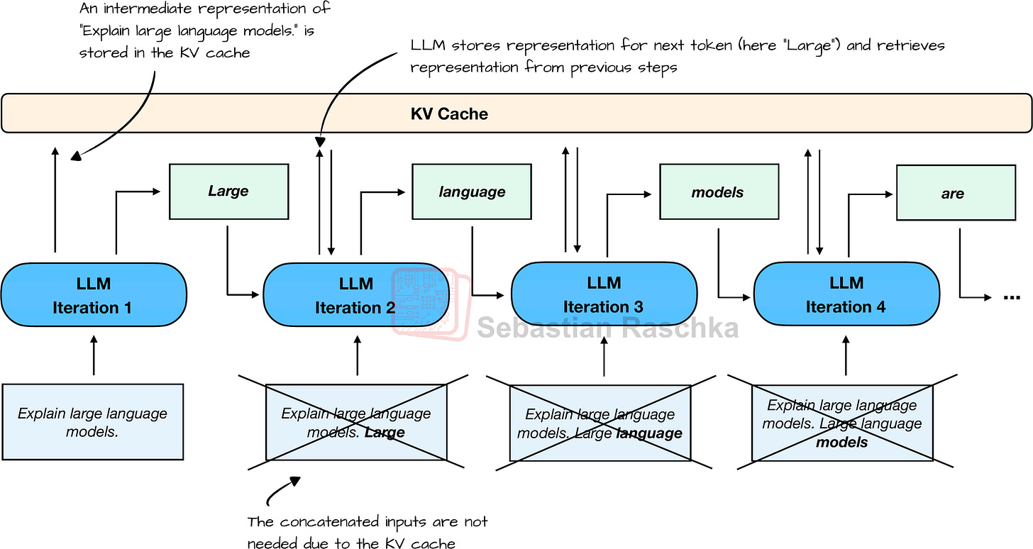
Now, the last puzzle piece we need is a text generation function wrapper to generate one word (token) at a time in typical LLM fashion, as illustrated in Figure 18:

Figure 18: The typical one-token-at-a-time text-generation pipeline of an LLM with KV cache.

The following code implements a text generation function with streaming, meaning that it is a Python generator that yields each token as it is generated, so that we can print it live:

def generate_text_basic_stream( model, token_ids, max_new_tokens, eos_token_id=None, context_size=None ): model.eval()

with torch.no_grad():
    cache = KVCache(n_layers=model.cfg["n_layers"])
    model.reset_kv_cache()

    # Prime the cache with the initial context
    logits = model(token_ids, cache=cache)

    for _ in range(max_new_tokens):
        next_token = torch.argmax(
            logits[:, -1], dim=-1, keepdim=True
        )

        if (eos_token_id is not None and
            torch.all(next_token == eos_token_id)):
            break

        yield next_token

        token_ids = torch.cat(
            [token_ids, next_token], dim=1
        )

        # Feed only the new token to the model;
        # cache handles history
        logits = model(next_token, cache=cache)

input_token_ids_tensor = torch.tensor( input_token_ids, device=device ).unsqueeze(0)

for token in generate_text_basic_stream( model=model, token_ids=input_token_ids_tensor, max_new_tokens=500, eos_token_id=tokenizer.eos_token_id ): token_id = token.squeeze(0).tolist() print( tokenizer.decode(token_id), end=““, flush=True )

The generated response is as follows:

Large language models (LLMs) are advanced artificial intelligence systems designed to generate human-like text. They are trained on vast amounts of text data, allowing them to understand and generate coherent, contextually relevant responses. LLMs are used in a variety of applications, including chatbots, virtual assistants, content generation, and more. They are powered by deep learning algorithms that enable them to process and generate text in a way that mimics human language.

Using the Reasoning Variant

In this section, we used the Qwen3 base model, which has not been fine-tuned or trained for reasoning (but thanks to the instruction and reasoning data in the pre-training data mix, it still follows instructions quite well).

To use the reasoning variant, you can replace USE_REASONING_MODEL=False with USE_REASONING_MODEL=True.

13 An Interactive Chat Interface

One step at a time, we implemented a fully-functional Qwen3 model that we can use for text generation tasks. However, while the PyTorch code serves educational purposes to solidify (and demystify) LLM concepts, it’s not the prettiest to look at as a primary user interface.

Optionally, I used the chainlit open-source library to create a quick and simple ChatGPT-like user interface for the code above. The code can be found here in my GitHub repository.

(Video/) Figure 19: An interactive chat interface for the Qwen3 model. This example shows the Qwen3 0.6B reasoning model.

14 Mixture-of-Experts Variant

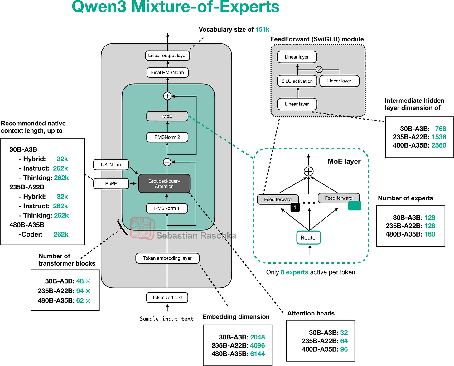
I realize that this article is already way too long. However, as a last point, I also wanted to also offer a few words about the Mixture-of-Experts (MoE) variants of Qwen3 shown in Figure 20.

Figure 20: The Qwen3 MoE architecture.

You are likely already familiar with MoE, but a quick recap may be helpful.

The core idea in MoE is to replace each FeedForward module in a transformer block with multiple expert layers, where each of these expert layers is also a FeedForward module. This means that we swap a single FeedForward block for multiple FeedForward blocks

So, replacing a single FeedForward block with multiple FeedForward blocks (as done in a MoE setup) substantially increases the model’s total parameter count. However, the key trick is that we don’t use (“activate”) all experts for every token. Instead, a router selects only a small subset of experts per token. (In the interest of time, or rather article space, I’ll cover the router in more detail another time.)

Because only a few experts are active at a time, MoE modules are often referred to as sparse, in contrast to dense modules that always use the full parameter set. However, the large total number of parameters via an MoE increases the capacity of the LLM, which means it can take up more knowledge during training. The sparsity keeps inference efficient, though, as we don’t use all the parameters at the same time.

So far, we implemented the dense Qwen3 architecture. Modifying it to also support the MoE variants is relatively simple and only requires a handful of changes. Note that this is not a very efficient implementation and more meant for illustration purposes, but it runs, albeit very slowly, on a single A100 (80 GB RAM).

First, we replace FeedForward by MoEFeedForward:

class MoEFeedForward(nn.Module): def init(self, cfg): super().__init__() self.num_experts_per_tok = cfg[“num_experts_per_tok”] self.num_experts = cfg[“num_experts”] self.gate = nn.Linear( cfg[“emb_dim”], cfg[“num_experts”], bias=False, dtype=cfg[“dtype”] )

    # meta device reduces memory pressure when
    # initializing before loading weights
    meta_device = torch.device("meta")

    self.fc1 = nn.ModuleList([
        nn.Linear(
            cfg["emb_dim"], cfg["moe_intermediate_size"],
            bias=False, dtype=cfg["dtype"],
            device=meta_device
        ) for _ in range(cfg["num_experts"])
    ])
    self.fc2 = nn.ModuleList([
        nn.Linear(
            cfg["emb_dim"], cfg["moe_intermediate_size"],
            bias=False, dtype=cfg["dtype"],
            device=meta_device
        ) for _ in range(cfg["num_experts"])
    ])
    self.fc3 = nn.ModuleList([
        nn.Linear(
            cfg["moe_intermediate_size"], cfg["emb_dim"],
            bias=False, dtype=cfg["dtype"],
            device=meta_device
        ) for _ in range(cfg["num_experts"])
    ])

def forward(self, x):
    b, seq_len, embed_dim = x.shape
    scores = self.gate(x)  # (b, t, num_experts)
    topk_scores, topk_indices = torch.topk(
        scores, self.num_experts_per_tok, dim=-1
    )
    topk_probs = torch.softmax(topk_scores, dim=-1)

    expert_outputs = []
    for e in range(self.num_experts):
        hidden = torch.nn.functional.silu(
            self.fc1[e](x)
        ) * self.fc2[e](x)
        out = self.fc3[e](hidden)
        expert_outputs.append(out.unsqueeze(-2))
    expert_outputs = torch.cat(
        expert_outputs, dim=-2
    )  # (b, t, num_experts, emb_dim)

    gating_probs = torch.zeros_like(scores)

    for i in range(self.num_experts_per_tok):
        indices = topk_indices[..., i:i+1]
        prob = topk_probs[..., i:i+1]
        gating_probs.scatter_(
            dim=-1, index=indices, src=prob
        )
    gating_probs = gating_probs.unsqueeze(
        -1
    )  # (b, t, num_experts, 1)

    # Weighted sum over experts
    y = (gating_probs * expert_outputs).sum(dim=-2)
    return y

Next, we have to make a small modification to the TransformerBlock:

class TransformerBlock(nn.Module): def init(self, cfg): super().__init__() self.att = GroupedQueryAttention( d_in=cfg[“emb_dim”], num_heads=cfg[“n_heads”], head_dim=cfg[“head_dim”], num_kv_groups=cfg[“n_kv_groups”], qk_norm=cfg[“qk_norm”], dtype=cfg[“dtype”] ) if cfg[“num_experts”] > 0: # NEW self.ff = MoEFeedForward(cfg) # NEW else: self.ff = FeedForward(cfg) self.norm1 = RMSNorm(cfg[“emb_dim”], eps=1e-6) self.norm2 = RMSNorm(cfg[“emb_dim”], eps=1e-6)

The config for the 30B-A3B variant looks like as follows, with 3 new keys added (“num_experts”, “num_experts_per_tok”, “moe_intermediate_size”):

QWEN3_CONFIG = { “vocab_size”: 151_936, “context_length”: 262_144, “emb_dim”: 2048, “n_heads”: 32, “n_layers”: 48, “head_dim”: 128, “qk_norm”: True, “n_kv_groups”: 4, “rope_base”: 10_000_000.0, “dtype”: torch.bfloat16, “num_experts”: 128, # NEW “num_experts_per_tok”: 8, # NEW “moe_intermediate_size”: 768, # NEW }

Finally, we have to modify the weight loading function with these new keys in mind:

def load_weights_into_qwen(model, param_config, params): # … # Feedforward weights if “num_experts” in param_config: # Load router (gating) weights block.ff.gate.weight = assign( block.ff.gate.weight, params[f”model.layers.{l}.mlp.gate.weight”], f”model.layers.{l}.mlp.gate.weight” ) # Load expert weights for e in range(param_config[“num_experts”]): prefix = f”model.layers.{l}.mlp.experts.{e}” block.ff.fc1[e].weight = assign( block.ff.fc1[e].weight, params[f”{prefix}.gate_proj.weight”], f”{prefix}.gate_proj.weight” ) block.ff.fc2[e].weight = assign( block.ff.fc2[e].weight, params[f”{prefix}.up_proj.weight”], f”{prefix}.up_proj.weight” ) block.ff.fc3[e].weight = assign( block.ff.fc3[e].weight, params[f”{prefix}.down_proj.weight”], f”{prefix}.down_proj.weight” ) # After assignin weights, # move expert layers from meta to CPU, # which is slower, # but allows the model to run on a single GPU block.ff.fc1[e] = block.ff.fc1[e].to(“cpu”) block.ff.fc2[e] = block.ff.fc2[e].to(“cpu”) block.ff.fc3[e] = block.ff.fc3[e].to(“cpu”) # …

You can find a standalone notebook with this MoE implementation here: standalone-qwen3-moe-plus-kvcache.ipynb

Conclusion

In this walkthrough, we stripped Qwen3 down to its core components and rebuilt it in plain PyTorch.

Along the way, we implemented all the essential building bloks: RMSNorm and QK-Norm normalization (and training stability), SwiGLU for for the feed-forward component, RoPE for positional encoding, grouped-query attention (GQA) for scalable memory use (esp. when used with a KV cache).

Once the building blocks were in place, we assembled them into a reusable Qwen3Model, loaded real, trained Qwen3 weights, implemented a text generation function, added a lightweight chat UI, and finally showed how the same design generalizes to Mixture-of-Experts (MoE) variants.

The code examples hopefully made these components more clear and tangible!

A final note: this code and write-up are meant for learning and experimentation. For production workloads, you will be much better off with optimized serving tools like Ollama (for simple local serving) or vLLM (for high-throughput, production-ready inference)

In any case, my hope is that this deep dive helps with your intuition for reading modern LLM papers and gives you confidence and motivation to tinker! 

Happy coding!

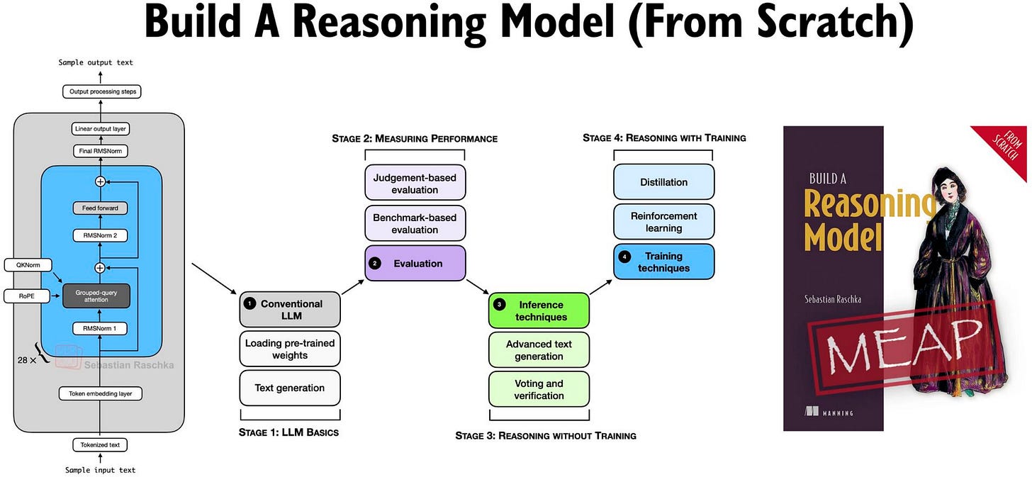
Build A Reasoning Model From Scratch

I have been working on something new: 📚 Build a Reasoning Model (From Scratch).

The first chapters just went live last week!

Figure 21: Visual overview of the Build a Reasoning Model (From Scratch) book.

Reasoning is one of the most exciting and important recent advances in improving LLMs, but it’s also one of the easiest to misunderstand if you only hear the term reasoning and read about it in theory. So, in this book, I am taking a hands-on approach to building a reasoning LLM from scratch.

If you liked “Build A Large Language Model (From Scratch)”, this book is written in a similar style in terms of building everything from scratch in pure PyTorch.

It’s a standalone book, but it basically continues where “Build A Large Language Model (From Scratch)” left off: we start with a pre-trained LLM (the Qwen3 base model we implemented in this article) and add reasoning methods (inference-time scaling, reinforcement learning, distillation) to improve its reasoning capabilities.

Here’s the table of contents to give you a better idea:

Chapter 1: Understanding reasoning models

Chapter 2: Generating text with a pre-trained LLM

Chapter 3: Evaluating reasoning models

Chapter 4: Improving reasoning with inference-time scaling

Chapter 5: Training reasoning models with reinforcement learning

Chapter 6: Distilling reasoning models for efficient reasoning

Chapter 7: Improving the reasoning pipeline and future research directions

Appendix A: References and further reading

Appendix B: Exercise solutions

Appendix C: LLM source code step by step

Appendix D: Loading larger models

Appendix E: KV-caching with batch support

If you want to check it out, it’s available for pre-order from the publisher here.

(How it works is you will get immediate access to the first chapters, each new chapter as it’s released, and the full book once complete.)

Thanks for subscribing to Ahead of AI! Your support means a great deal and is tremendously helpful in continuing this journey as an independent researcher. Thank you!